cartopy が依存している pykdtree について何か書こうと思ってたら、興味の中心が imshow の方に移動してた。
matplotlib における imshow というのはこれは、無論「jpeg とかを貼り付けられるんだぜぃ」という見方でも間違ってはいないんだけれど、「Matrix Plotting Library」であるところの matplotlib としてはこれは、2-D array の列が x、行が y に直接対応する場合に使う、いわば pcolor のショートカットのような、つまりはあくまでも「行列可視化」のインターフェイスなわけである。たとえば最もシンプルにはこういうことだ:
1 # -*- coding: utf-8 -*-
2 import numpy as np
3 import matplotlib.pyplot as plt
4
5
6 def main():
7 fig = plt.figure()
8 fig.set_size_inches(16.53, 11.69)
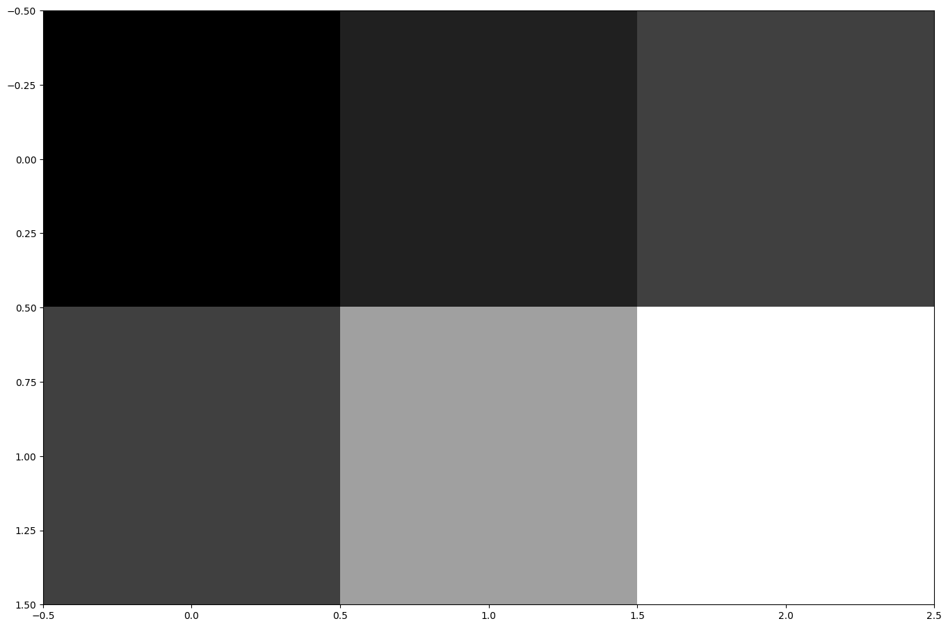
9 twodimarr = np.array([
10 [10, 20, 30,],
11 [30, 60, 90,],
12 ])
13 ax1 = fig.add_subplot()
14 ax1.imshow(twodimarr, cmap="gray")
15 plt.savefig("exam_imshow_00.png", bbox_inches="tight")
16 plt.close(fig)
17
18
19 if __name__ == '__main__':
20 main()
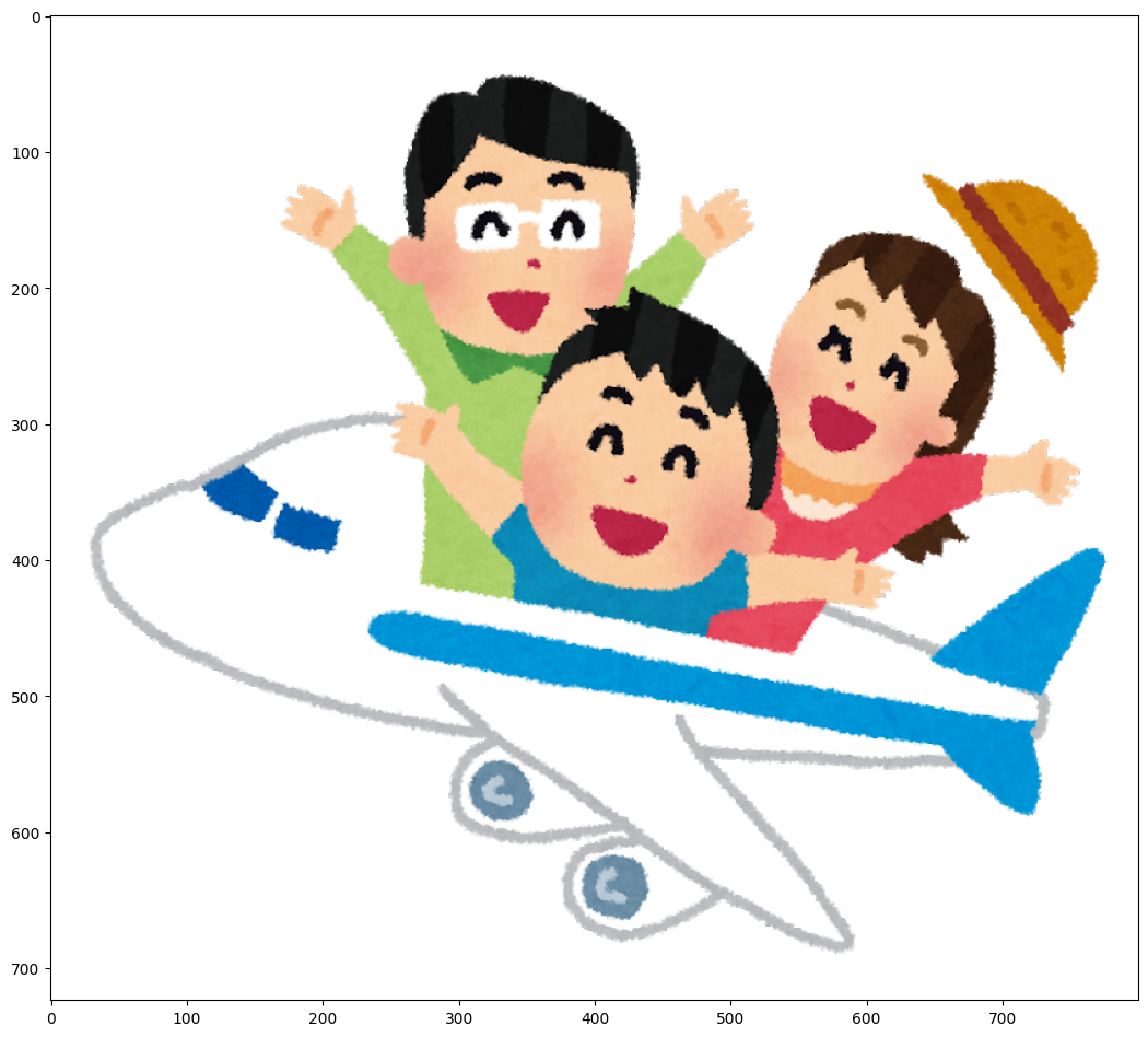
「jpeg だの png だってただの二次元行列なのさぁ」てことなわけだ:
 1 # -*- coding: utf-8 -*-
 2 import numpy as np
 3 import matplotlib.pyplot as plt
 4
 5
 6 def main():
 7     fig = plt.figure()
 8     fig.set_size_inches(16.53, 11.69)
 9     ax1 = fig.add_subplot()
10     img = plt.imread("family_airplane_travel.png")  # 「いらすとや」より。
11     ax1.imshow(img)
12     plt.savefig("exam_imshow_01.png", bbox_inches="tight")
13     plt.close(fig)
14
15
16 if __name__ == '__main__':
17     main()
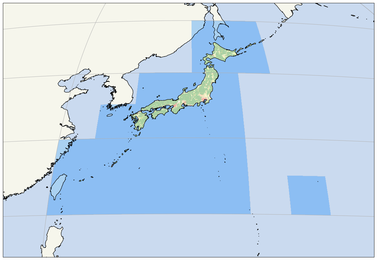
なので、cartopy でも imshow 出来る、ということのその意味は、気象予測グリッドデータと地図の重ね合わせの例に求めるのと同じく、「座標系変換を良きに計らってもらう」ことである:
 1 # -*- coding: utf-8 -*-
 2 import numpy as np
 3 import matplotlib.pyplot as plt
 4 import cartopy.crs as ccrs
 5 import cartopy.feature as cfeature
 6
 7
 8 def main():
 9     fig = plt.figure()
10     fig.set_size_inches(16.53, 11.69)
11     ext = [126.0 + 12, 146.5 - 4, 25.0 + 9, 46.5 - 9]
12     crs = ccrs.Geostationary((ext[0] + ext[1]) / 2)
13     ax1 = fig.add_subplot(projection=crs)
14     ax1.set_extent(ext, ccrs.PlateCarree())
15     ax1.coastlines(resolution="10m")
16     ax1.gridlines()
17     ax1.add_feature(cfeature.OCEAN, alpha=0.5)
18     ax1.add_feature(cfeature.LAND, alpha=0.5)
19     #
20     img = plt.imread("family_airplane_travel.png")
21     ax1.imshow(
22         img,
23         origin='upper',
24         extent=[ext[0] + 2.75, ext[1] - 0.25, ext[2] + 0.5, ext[3] - 2.0],
25         transform=ccrs.PlateCarree(),
26         zorder=9)
27     #
28     plt.savefig("exam_imshow_02_geoaxis.png", bbox_inches="tight")
29     plt.close(fig)
30
31
32 if __name__ == '__main__':
33     main()
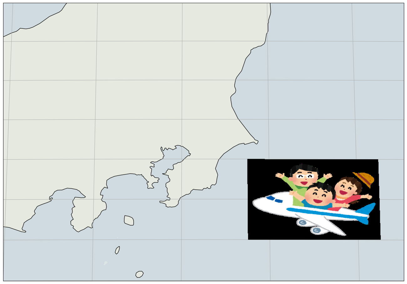
まぁ imshow の話としては単にこれだけ。ただ、使い方の注意点はあって、ワタシが苦労したのは transform と zorder (or alpha)。後者はもちろん「隠れちゃってみえねー」問題なので、わかってしまえばまぁ「あぁよくあるヤツだ」と思った。前者ね。ほかのもそうだったんで、そのつもりで取り組めば良かったんだけれど、「transform を指定しないで」試しちゃったのよね。これだと見える範囲内に正しく描画されない。それと、set_extent のタイミングにも注意、これで悩んだ人もいる。
GeoTIFF をダイレクトに描画出来るようには imshow は拡張されてないと思うが、geotiff タグを不自由なく読み解けるんであれば、別に大問題でもない。まぁ「めっさ簡単だ」とは言わんけどね:
1 # -*- coding: utf-8 -*-
2 import struct
3 from PIL import Image
4 import numpy as np
5 import matplotlib.pyplot as plt
6 import cartopy.crs as ccrs
7 import cartopy.feature as cfeature
8 #from cartopy.io.img_tiles import Stamen, GoogleTiles
9
10
11 _tags = {
12 # https://www.awaresystems.be/imaging/tiff/tifftags/modelpixelscaletag.html
13 33550: "ModelPixelScale", # (ScaleX, ScaleY, ScaleZ)
14
15 # https://www.awaresystems.be/imaging/tiff/tifftags/modeltiepointtag.html
16 33922: "ModelTiepoint", # (...,I,J,K, X,Y,Z...)
17
18 # https://www.awaresystems.be/imaging/tiff/tifftags/modeltransformationtag.html
19 34264: "ModelTransformation", # double*16
20
21 # https://www.awaresystems.be/imaging/tiff/tifftags/geokeydirectorytag.html
22 34735: "GeoKeyDirectory",
23
24 # https://www.awaresystems.be/imaging/tiff/tifftags/geodoubleparamstag.html
25 34736: "GeoDoubleParams",
26
27 # https://www.awaresystems.be/imaging/tiff/tifftags/geoasciiparamstag.html
28 34737: "GeoAsciiParams",
29 }
30
31
32 _keys = {
33 1024: 'GTModelTypeGeoKey',
34 1025: 'GTRasterTypeGeoKey',
35 1026: 'GTCitationGeoKey',
36 2048: 'GeographicTypeGeoKey',
37 2049: 'GeogCitationGeoKey',
38 2050: 'GeogGeodeticDatumGeoKey',
39 2051: 'GeogPrimeMeridianGeoKey',
40 2052: 'GeogLinearUnitsGeoKey',
41 2053: 'GeogLinearUnitSizeGeoKey',
42 2054: 'GeogAngularUnitsGeoKey',
43 2055: 'GeogAngularUnitsSizeGeoKey',
44 2056: 'GeogEllipsoidGeoKey',
45 2057: 'GeogSemiMajorAxisGeoKey',
46 2058: 'GeogSemiMinorAxisGeoKey',
47 2059: 'GeogInvFlatteningGeoKey',
48 2060: 'GeogAzimuthUnitsGeoKey',
49 2061: 'GeogPrimeMeridianLongGeoKey',
50 2062: 'GeogTOWGS84GeoKey',
51 3059: 'ProjLinearUnitsInterpCorrectGeoKey', # GDAL
52 3072: 'ProjectedCSTypeGeoKey',
53 3073: 'PCSCitationGeoKey',
54 3074: 'ProjectionGeoKey',
55 3075: 'ProjCoordTransGeoKey',
56 3076: 'ProjLinearUnitsGeoKey',
57 3077: 'ProjLinearUnitSizeGeoKey',
58 3078: 'ProjStdParallel1GeoKey',
59 3079: 'ProjStdParallel2GeoKey',
60 3080: 'ProjNatOriginLongGeoKey',
61 3081: 'ProjNatOriginLatGeoKey',
62 3082: 'ProjFalseEastingGeoKey',
63 3083: 'ProjFalseNorthingGeoKey',
64 3084: 'ProjFalseOriginLongGeoKey',
65 3085: 'ProjFalseOriginLatGeoKey',
66 3086: 'ProjFalseOriginEastingGeoKey',
67 3087: 'ProjFalseOriginNorthingGeoKey',
68 3088: 'ProjCenterLongGeoKey',
69 3089: 'ProjCenterLatGeoKey',
70 3090: 'ProjCenterEastingGeoKey',
71 3091: 'ProjFalseOriginNorthingGeoKey',
72 3092: 'ProjScaleAtNatOriginGeoKey',
73 3093: 'ProjScaleAtCenterGeoKey',
74 3094: 'ProjAzimuthAngleGeoKey',
75 3095: 'ProjStraightVertPoleLongGeoKey',
76 3096: 'ProjRectifiedGridAngleGeoKey',
77 4096: 'VerticalCSTypeGeoKey',
78 4097: 'VerticalCitationGeoKey',
79 4098: 'VerticalDatumGeoKey',
80 4099: 'VerticalUnitsGeoKey',
81 }
82
83
84 def getgeotiffdata(img):
85 result = {}
86
87 if not hasattr(img, "tag"):
88 img = Image.open(img)
89 tagdata = img.tag.tagdata
90
91 # ModelPixelScale
92 if 33550 in tagdata:
93 result[_tags[33550]] = struct.unpack(
94 "<3d", tagdata[33550])
95
96 # ModelTiepoint
97 if 33922 in tagdata:
98 result[_tags[33922]] = struct.unpack(
99 "<{}d".format(len(tagdata[33922]) // 8), tagdata[33922])
100
101 # ModelTransformation
102 if 34264 in tagdata:
103 result[_tags[34264]] = struct.unpack(
104 "<{}d".format(len(tagdata[34264]) // 8), tagdata[34264])
105
106 # GeoKeyDirectory
107 # GeoDoubleParams
108 # GeoAsciiParams
109 if 34735 in tagdata:
110 inner = result[_tags[34735]] = [{}, {}]
111 #
112 gkd = struct.unpack("<{}H".format(len(tagdata[34735]) // 2), tagdata[34735])
113 gkd = [gkd[i:i + 4] for i in range(0, len(gkd), 4)]
114 KeyDirectoryVersion, KeyRevision, KeyRevisionMinor = gkd.pop(0)[:-1]
115 inner[0]["KeyDirectoryVersion"] = KeyDirectoryVersion
116 inner[0]["KeyRevision"] = KeyRevision
117 inner[0]["KeyRevisionMinor"] = KeyRevisionMinor
118 #
119 for keyid, tagid, count, offset in gkd:
120 if tagid == 0:
121 value = offset
122 else:
123 if tagid == 34736:
124 value = tagdata[tagid]
125 value = struct.unpack("<{}d".format(len(value) // 8), value)
126 elif tagid == 34737:
127 value = tagdata[tagid][offset:offset + count]
128 value = value.decode()
129 if value[-1] == "|":
130 value = value[:-1]
131 else:
132 raise NotImplementedError("sorry")
133 inner[1][_keys.get(keyid, keyid)] = value
134 return result, img.size
135
136
137 def gettransforms(geotiffdata):
138 """
139 build modeltransformation from modelpixelscale, and modeltiepoint
140 """
141 transforms = []
142 if "ModelPixelScale" in geotiffdata and "ModelTiepoint" in geotiffdata:
143 # see "B.6. GeoTIFF Tags for Coordinate Transformations"
144 # in https://earthdata.nasa.gov/files/19-008r4.pdf.
145 sx, sy, sz = geotiffdata["ModelPixelScale"]
146 tiepoints = geotiffdata["ModelTiepoint"]
147 for tp in range(0, len(tiepoints), 6):
148 i, j, k, x, y, z = tiepoints[tp:tp + 6]
149 transforms.append([
150 [sx, 0.0, 0.0, x - i * sx],
151 [0.0, -sy, 0.0, y + j * sy],
152 [0.0, 0.0, sz, z - k * sz],
153 [0.0, 0.0, 0.0, 1.0]])
154 return transforms
155
156
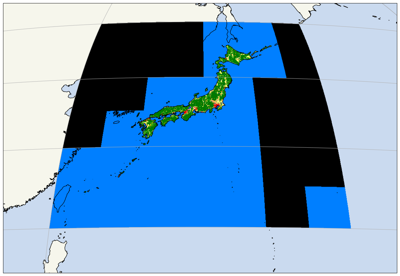
157 def main():
158 # 国土地理院配布の地勢図
159 # see "Geospatial Information Authority of Japan Website Terms of Use",
160 # http://www.gsi.go.jp/ENGLISH/page_e30286.html
161 geotiffdata, (width, height) = getgeotiffdata(
162 "gm-jpn-lu_u_1_1/jpn/lu.tif")
163 #
164 transforms = gettransforms(geotiffdata)
165 bb_tl = np.dot(transforms, [0, 0, 0, 1])[0,:2] # top-left
166 bb_br = np.dot(transforms, [width, height, 0, 1])[0,:2] # bottom-right
167 #
168 fig = plt.figure()
169 fig.set_size_inches(16.53, 11.69)
170 crs = ccrs.Geostationary((bb_br[0] + bb_tl[0]) / 2)
171 #tiler = GoogleTiles(style="satellite")
172 #crs = tiler.crs
173 ax1 = fig.add_subplot(projection=crs)
174 ax1.set_extent(
175 [bb_tl[0] - 5, bb_br[0] + 5, bb_br[1] - 5, bb_tl[1] + 5],
176 ccrs.PlateCarree())
177 #ax1.add_image(tiler, 5, alpha=0.5)
178 ax1.coastlines(resolution="10m")
179 ax1.gridlines()
180 ax1.add_feature(cfeature.OCEAN, alpha=0.5)
181 ax1.add_feature(cfeature.LAND, alpha=0.5)
182 #
183 img = plt.imread("gm-jpn-lu_u_1_1/jpn/lu.tif")
184 ax1.imshow(
185 img,
186 origin='upper',
187 extent=[bb_tl[0], bb_br[0], bb_br[1], bb_tl[1]],
188 transform=ccrs.PlateCarree(),
189 zorder=-1)
190
191 plt.savefig("exam_imshow_03_geoaxis_geotiff.png", bbox_inches="tight")
192 plt.close(fig)
193
194
195 if __name__ == '__main__':
196 main()
ここでも触れておいたが、tifffile を使えばかなり楽出来る:
1 # -*- coding: utf-8 -*-
2 from PIL import Image
3 import numpy as np
4 import matplotlib.pyplot as plt
5 import cartopy.crs as ccrs
6 import cartopy.feature as cfeature
7 import tifffile
8
9
10 def getgeotiffdata(img):
11 return tifffile.TiffFile(img).pages[0].geotiff_tags, Image.open(img).size
12
13
14 def gettransforms(geotiffdata):
15 """
16 build modeltransformation from modelpixelscale, and modeltiepoint
17 """
18 transforms = []
19 if "ModelPixelScale" in geotiffdata and "ModelTiepoint" in geotiffdata:
20 # see "B.6. GeoTIFF Tags for Coordinate Transformations"
21 # in https://earthdata.nasa.gov/files/19-008r4.pdf.
22 sx, sy, sz = geotiffdata["ModelPixelScale"]
23 tiepoints = geotiffdata["ModelTiepoint"]
24 for tp in range(0, len(tiepoints), 6):
25 i, j, k, x, y, z = tiepoints[tp:tp + 6]
26 transforms.append([
27 [sx, 0.0, 0.0, x - i * sx],
28 [0.0, -sy, 0.0, y + j * sy],
29 [0.0, 0.0, sz, z - k * sz],
30 [0.0, 0.0, 0.0, 1.0]])
31 return transforms
32
33
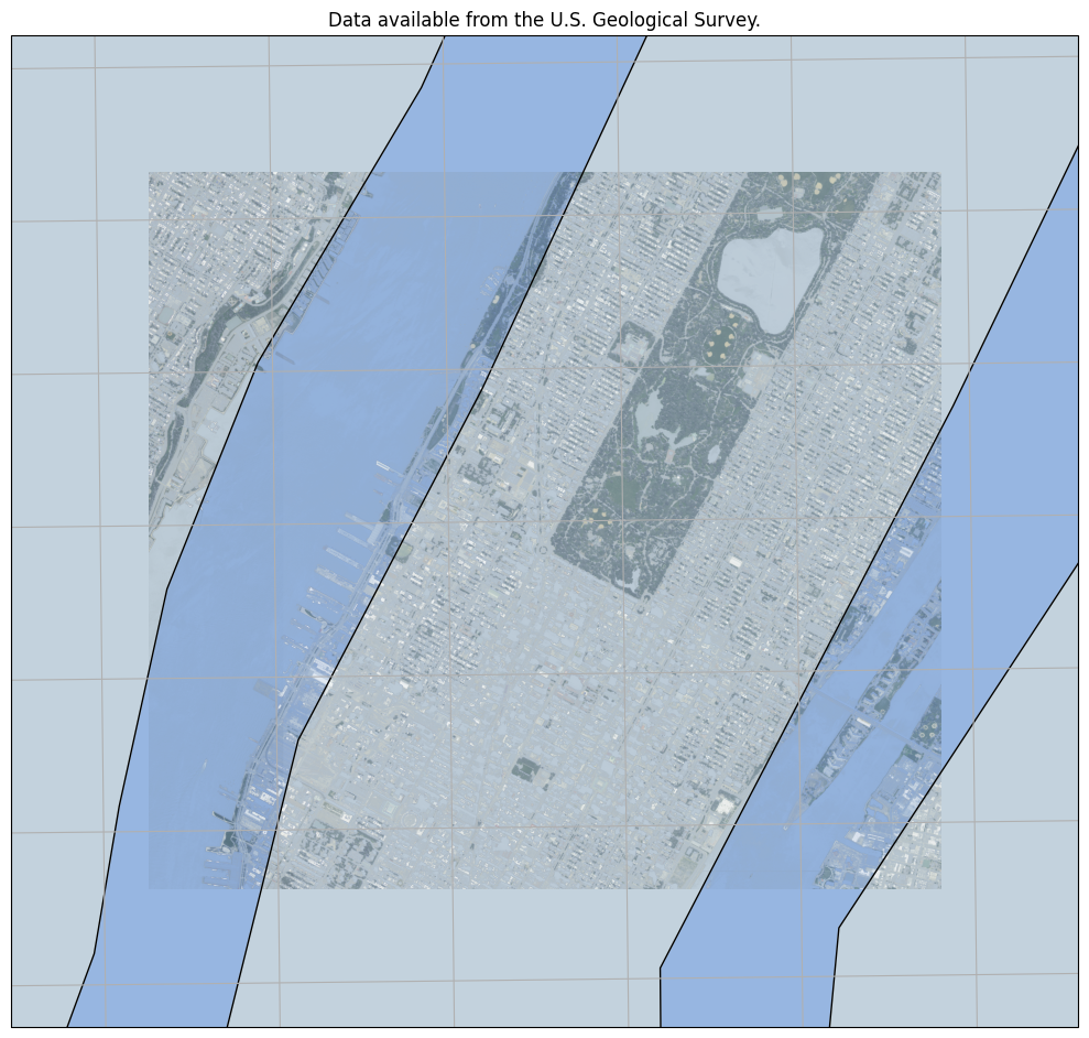
34 def main():
35 # Kelsey Jordahl (Enthought)'s DATA_CREDITS.md says:
36 # The file `manhattan.tif` is a [Digital Orthophoto Quadrangle (DOQ)]
37 # (https://lta.cr.usgs.gov/DOQs) from the USGS and in the public domain
38 # ([direct link](http://earthexplorer.usgs.gov/metadata/1131/DI00000000845784)).
39 # They [request](https://lta.cr.usgs.gov/citation) the following attribution
40 # statement when using thir data:
41 # "Data available from the U.S. Geological Survey."
42 geotiffdata, (width, height) = getgeotiffdata(
43 "data/manhattan.tif")
44 #
45 transforms = gettransforms(geotiffdata)
46 bb_tl = np.dot(transforms, [0, 0, 0, 1])[0,:2] # top-left
47 bb_br = np.dot(transforms, [width, height, 0, 1])[0,:2] # bottom-right
48 #
49 fig = plt.figure()
50 fig.set_size_inches(16.53, 11.69)
51 crs = ccrs.UTM("18N")
52 ax1 = fig.add_subplot(projection=crs)
53 ax1.set_extent(
54 [bb_tl[0] - 10**3, bb_br[0] + 10**3, bb_br[1] - 10**3, bb_tl[1] + 10**3],
55 crs)
56 ax1.coastlines(resolution="10m")
57 ax1.gridlines()
58 ax1.add_feature(cfeature.OCEAN, alpha=0.5)
59 ax1.add_feature(cfeature.LAND, alpha=0.5)
60 #
61 img = plt.imread("data/manhattan.tif")
62 ax1.imshow(
63 img,
64 origin='upper',
65 extent=[bb_tl[0], bb_br[0], bb_br[1], bb_tl[1]],
66 transform=crs,
67 alpha=0.8)
68 ax1.set_title("Data available from the U.S. Geological Survey.")
69 plt.savefig("exam_imshow_04_geoaxis_geotiff_2.png", bbox_inches="tight")
70 plt.close(fig)
71
72
73 if __name__ == '__main__':
74 main()
なお、「GeoTIFFを扱えるステキなもの」として GDAL をオススメられたのなら、かなり待つがいい。GDAL の導入は果てしなくバカバカしい。GIS に関するありとあらゆることをしたいと思わない限りは、なるべく依存しないで済むように行動するのがベター。先日書いたように、目下「ミーツー運動勃発中」。まぁ GIS 関連はどのプロジェクトも結構乱雑で荒れがちではあるんだけれど、やはりワタシも GDAL に対する印象が一番ヒドい。依存関係がかなりオカシイ、というか、たぶんね、「整理する努力が欠けている」的なことなんだと思うわ。運動首謀者の言う「ナイトメア」は、ほんとワタシもそう思う、てこと。
作者(みーつぅな首謀者そのヒト)が「未完なので応援してちょ」と言ってるので少し注意深く経過観察する必要はあるものの、今の「giotiff 描画にまつわるエトセトラ」について、geotiff は検討して良いと思う。ただし、まだ読み込みしか出来ない。「ロードマップ」として writer も挙げているので、待ってれば作られるはずではある。(ただ、まだ試してないけどおそらく tifffile で書き出しも出来てしまうので、それで出来るのであれば、そちらを直接使えばいいのだろう。geotiff 専用なのかどうかの違いとなるはずなので、煩雑さに差が出る、という程度だろう、きっと。)
ここでちょっと補足というか「蛇足」をついでに。「GeoTIFF」は、つまりは TIFF の仕様を利用して GIS のためのメタデータをバイナリとして埋め込む、という仕様なわけだけれど、「そのメタデータのための入力」として、もしくは「その存在そのものがメタデータとして機能」する「ESRI World File」がある。GDAL のコマンドラインツールはこれを入力として GeoTIFF を作ったりも出来る(はず、遠い記憶によれば)し、「(GeoTIFF ではない)TIFF + ESRI World File」のペアを認識出来るツールもある(と思う)。
思う、とか、確か、とか曖昧で申し訳ないが、個人的に OGR/GDAL には一切手を出したくなくてな。確かめる作業そのものが苦痛なの。実際ワタシが自分で試したのは、もう10年も前になるのだが、やり直したくないし。
ともあれ、今ここで言いたいのは、「ESRI World File を手持ち」の場合に、そちらを読む手もある、という話。事実、国土地理院から入手可能なものは、tfw ファイルが一緒についてくる:
1                    0.00833333376795
2                    0.00000000000000
3                    0.00000000000000
4                   -0.00833333376795
5                  120.00416564941406
6                   49.99583374708891
これを読み解くと、こうなる:
1 'ModelPixelScale': [0.00833333376795, 0.00833333376795, 0.0]
2 'ModelTiepoint': [0.0, 0.0, 0.0, 120.00416564941406, 49.99583374708891, 0.0]
EXIF データとして埋め込まれてないならこれを読むしかないということにはなるが、バイナリデータを読み解くのが面倒だ、という時には、こちらを読むのも手かもしれない。(実際、ワタシが上で書いた Pillow だけで読んでる実装は実はエンディアンの扱いをサボっていて、Big-endian で収められてる場合に間違ったデータ解釈をしでかしてしまう。そうなるくらいなら、こちらを読んでしまうってのはアリ。)
ついでなので、WMS もやっとく。add_wms を使うためには、OWSLib を別途インストールする必要がある。「OGC 策定の WMS (Web Map Serice API)」の良し悪しはともかくとして、OWSLib はそれ単独としてシンプルで使いやすい:
 1 >>> from owslib.wms import WebMapService
 2 >>> wms = WebMapService('http://vmap0.tiles.osgeo.org/wms/vmap0')
 3 >>> img = wms.getmap(
 4 ...     layers=["basic", "country_01"],
 5 ...     srs="EPSG:4326",
 6 ...     bbox=[126.0 + 12, 25.0 + 9, 146.5 - 4, 46.5 - 9],
 7 ...     size=(1280, 720),
 8 ...     format='image/jpeg', transparent=True)
 9 >>> out = open("osgeo_wms_tiles__basic__country_01.jpg", "wb")
10 >>> out.write(img.read())
11 38650
12 >>> out.close()
で、インストールしてあれば、cartopy で add_wms を使える:
 1 # -*- coding: utf-8 -*-
 2 from PIL import Image
 3 import numpy as np
 4 import matplotlib.pyplot as plt
 5 import cartopy.crs as ccrs
 6 import tifffile
 7
 8
 9 def getgeotiffdata(img):
10     return tifffile.TiffFile(img).pages[0].geotiff_tags, Image.open(img).size
11
12
13 def gettransforms(geotiffdata):
14     """
15     build modeltransformation from modelpixelscale, and modeltiepoint
16     """
17     transforms = []
18     if "ModelPixelScale" in geotiffdata and "ModelTiepoint" in geotiffdata:
19         # see "B.6. GeoTIFF Tags for Coordinate Transformations"
20         # in https://earthdata.nasa.gov/files/19-008r4.pdf.
21         sx, sy, sz = geotiffdata["ModelPixelScale"]
22         tiepoints = geotiffdata["ModelTiepoint"]
23         for tp in range(0, len(tiepoints), 6):
24             i, j, k, x, y, z = tiepoints[tp:tp + 6]
25             transforms.append([
26                 [sx, 0.0, 0.0, x - i * sx],
27                 [0.0, -sy, 0.0, y + j * sy],
28                 [0.0, 0.0, sz, z - k * sz],
29                 [0.0, 0.0, 0.0, 1.0]])
30     return transforms
31
32
33 def main():
34     # Kelsey Jordahl (Enthought)'s DATA_CREDITS.md says:
35     #     The file `landsat.tif` was derived from Landsat 8 data downloaded
36     #     through [Libra](https://libra.developmentseed.org) and served by
37     #     [AWS](http://aws.amazon.com/public-data-sets/landsat). The original
38     #     file is [LC80420272015130LGN00](http://landsat-pds.s3.amazonaws.com/
39     #     L8/042/027/LC80420272015130LGN00/index.html) from 10 May 2015 and
40     #     was processed with [landsat-util](https://github.com/developmentseed/
41     #     landsat-util) to reduce the number of bands. The Landsat 8 files are
42     #     in the public domain, and I hereby release my changes in the file
43     #     `landsat.tif` to the public domain under
44     #     [CC0](https://creativecommons.org/publicdomain/zero/1.0).
45     geotiffdata, (width, height) = getgeotiffdata(
46         "data/landsat.tif")
47     #
48     #print(geotiffdata)
49     transforms = gettransforms(geotiffdata)
50     bb_tl = np.dot(transforms, [0, 0, 0, 1])[0, :2]  # top-left
51     bb_br = np.dot(transforms, [width, height, 0, 1])[0, :2]  # bottom-right
52     #
53     #tiler = GoogleTiles(style="street")
54     fig = plt.figure()
55     fig.set_size_inches(16.53, 11.69)
56     crs = ccrs.epsg("3857")
57     ax1 = fig.add_subplot(projection=crs)
58     ax1.set_extent(
59         [bb_tl[0] - 10**4, bb_br[0] + 10**4, bb_br[1] - 10**4, bb_tl[1] + 10**4],
60         crs)
61     #ax1.add_wms(
62     #    wms='http://vmap0.tiles.osgeo.org/wms/vmap0',
63     #    layers=["basic",], alpha=0.5)
64     #ax1.add_wms(
65     #    wms='https://ows.terrestris.de/osm/service',
66     #    layers=["TOPO-OSM-WMS",], alpha=0.5)
67     ax1.add_wms(
68         wms='https://ows.terrestris.de/osm/service',
69         layers=["OSM-WMS",], alpha=0.5)
70     #ax1.add_image(tiler, 9)
71     #
72     img = plt.imread("data/landsat.tif")
73     ax1.imshow(
74         img,
75         origin='upper',
76         extent=[bb_tl[0], bb_br[0], bb_br[1], bb_tl[1]],
77         transform=crs,
78         zorder=-1)
79     plt.savefig("exam_imshow_04_geoaxis_geotiff_2-2.png", bbox_inches="tight")
80     plt.close(fig)
81
82
83 if __name__ == '__main__':
84     main()
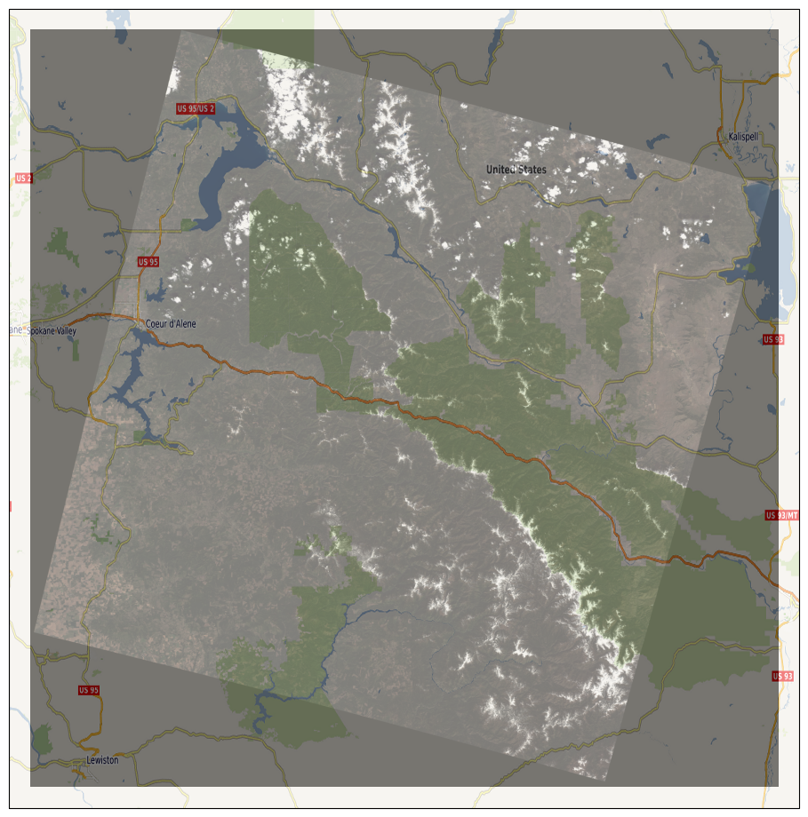
GoogleTiles や Stamen で add_image するのと比較しての使用感は、python コードとしての見かけはほとんど変わらない。無論サーバのインターフェイスが OSM らのものと同じではなく、出来ることも少し違うけれど、ほとんどは単に「選択の自由が広がっただけ」だと感じれるんではないかと思う。
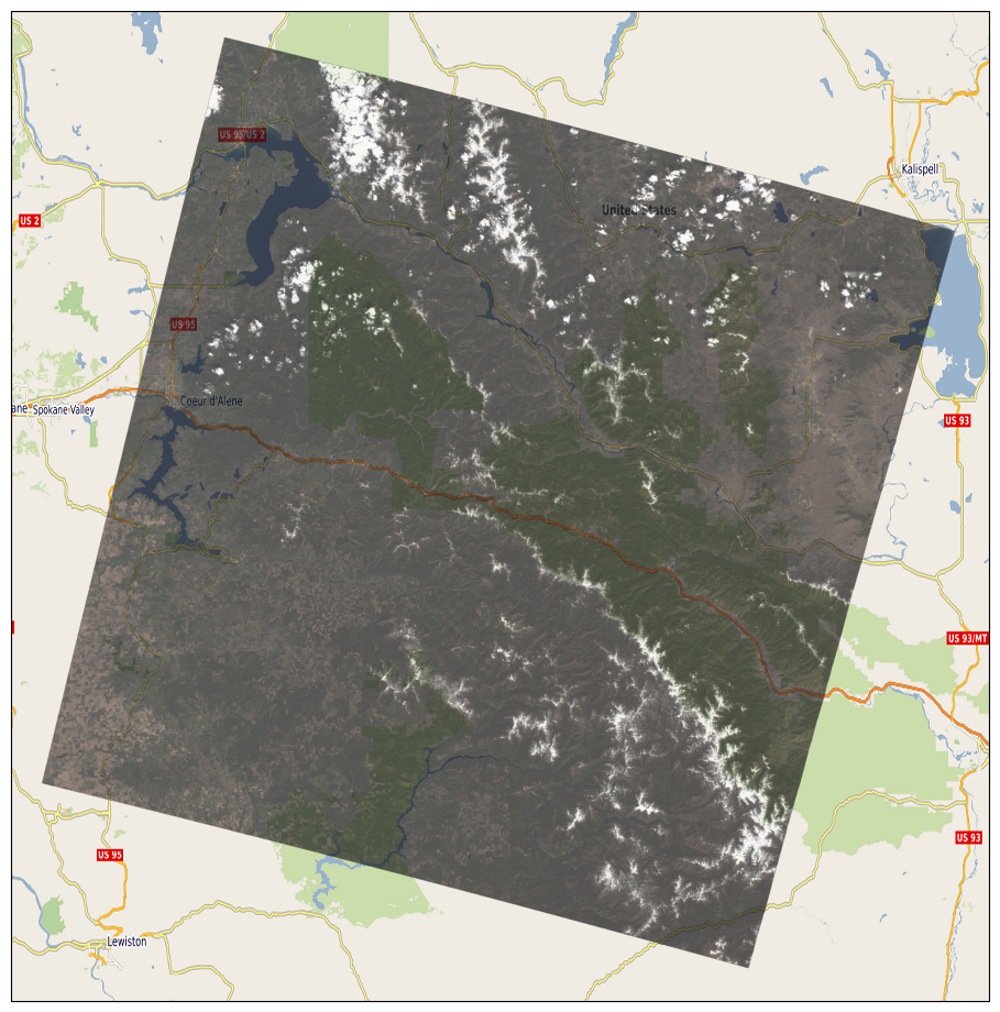
「スケスケろ、いやーんお代官様ごしょうにございますぅ」問題が相も変わらず鬱陶しいけれど、(4)で例にしたみたいな、我々が関与できない部分の振る舞いに頼らざるを得ないのとは違って、今の場合はなんせ「イメージデータそのもの」を(numpy.ndarray で)手持ちなので、いっそ自力で RGBA を作ってしまえばいいんじゃないか?:
 1 # -*- coding: utf-8 -*-
 2 from PIL import Image
 3 import numpy as np
 4 import matplotlib.pyplot as plt
 5 import cartopy.crs as ccrs
 6 import tifffile
 7
 8
 9 def getgeotiffdata(img):
10     return tifffile.TiffFile(img).pages[0].geotiff_tags, Image.open(img).size
11
12
13 def gettransforms(geotiffdata):
14     """
15     build modeltransformation from modelpixelscale, and modeltiepoint
16     """
17     transforms = []
18     if "ModelPixelScale" in geotiffdata and "ModelTiepoint" in geotiffdata:
19         # see "B.6. GeoTIFF Tags for Coordinate Transformations"
20         # in https://earthdata.nasa.gov/files/19-008r4.pdf.
21         sx, sy, sz = geotiffdata["ModelPixelScale"]
22         tiepoints = geotiffdata["ModelTiepoint"]
23         for tp in range(0, len(tiepoints), 6):
24             i, j, k, x, y, z = tiepoints[tp:tp + 6]
25             transforms.append([
26                 [sx, 0.0, 0.0, x - i * sx],
27                 [0.0, -sy, 0.0, y + j * sy],
28                 [0.0, 0.0, sz, z - k * sz],
29                 [0.0, 0.0, 0.0, 1.0]])
30     return transforms
31
32
33 def main():
34     # Kelsey Jordahl (Enthought)'s DATA_CREDITS.md says:
35     #     The file `landsat.tif` was derived from Landsat 8 data downloaded
36     #     through [Libra](https://libra.developmentseed.org) and served by
37     #     [AWS](http://aws.amazon.com/public-data-sets/landsat). The original
38     #     file is [LC80420272015130LGN00](http://landsat-pds.s3.amazonaws.com/
39     #     L8/042/027/LC80420272015130LGN00/index.html) from 10 May 2015 and
40     #     was processed with [landsat-util](https://github.com/developmentseed/
41     #     landsat-util) to reduce the number of bands. The Landsat 8 files are
42     #     in the public domain, and I hereby release my changes in the file
43     #     `landsat.tif` to the public domain under
44     #     [CC0](https://creativecommons.org/publicdomain/zero/1.0).
45     geotiffdata, (width, height) = getgeotiffdata(
46         "data/landsat.tif")
47     #
48     #print(geotiffdata)
49     transforms = gettransforms(geotiffdata)
50     bb_tl = np.dot(transforms, [0, 0, 0, 1])[0, :2]  # top-left
51     bb_br = np.dot(transforms, [width, height, 0, 1])[0, :2]  # bottom-right
52     #
53     fig = plt.figure()
54     fig.set_size_inches(16.53, 11.69)
55     crs = ccrs.epsg("3857")
56     ax1 = fig.add_subplot(projection=crs)
57     ax1.set_extent(
58         [bb_tl[0] - 10**4, bb_br[0] + 10**4, bb_br[1] - 10**4, bb_tl[1] + 10**4],
59         crs)
60     ax1.add_wms(
61         wms='https://ows.terrestris.de/osm/service',
62         layers=["OSM-WMS",])
63     #
64     img = plt.imread("data/landsat.tif")
65     alpha = np.full((img.shape[0], img.shape[1], 1), int(0.7 * 255))
66     zeroe = (img == 0)
67     zeroe = np.logical_and(zeroe[:,:,0], zeroe[:,:,1], zeroe[:,:,2])
68     alpha[np.where(zeroe)] = 0
69     img_rgba = np.concatenate((img, alpha), axis=2)
70     ax1.imshow(
71         img_rgba,
72         origin='upper',
73         extent=[bb_tl[0], bb_br[0], bb_br[1], bb_tl[1]],
74         transform=crs)
75     plt.savefig("exam_imshow_04_geoaxis_geotiff_2-3.png", bbox_inches="tight")
76     plt.close(fig)
77
78
79 if __name__ == '__main__':
80     main()
をぉ、よしよし、とほくそ笑んだのも束の間、同じやり口で「国土地理院のやーつ」をやってみても、全く透けずに、とても弱っていた。
まず「手始め」のつまづきとしては、gm-jpn-lu_u_1_1/jpn/lu.tif そのものが実はアルファチャンネルを持っている(つまり RGBA)であるということなのだが、それ自体は別に難しいことじゃない:
1 img = plt.imread("gm-jpn-lu_u_1_1/jpn/lu.tif")[:,:,:3]
スケスケないパターンは「not same_projection」の場合、なので、subplot の projection として Geostationary、imshow の transform としてそれ以外を使ってると、スケスケない可能性が出てくる。結局 cartopy/mpl/geoaxes.py に print 入れまくってやっとわかったんだけど、「As a workaround to a matplotlib limitation」が悪さしてしまうのね。色々やってみたのだが、以下が正解かしらね:
 1 # -*- coding: utf-8 -*-
 2 from PIL import Image
 3 import numpy as np
 4 import matplotlib.pyplot as plt
 5 import cartopy.crs as ccrs
 6 import cartopy.feature as cfeature
 7 import tifffile
 8
 9
10 def getgeotiffdata(img):
11     return tifffile.TiffFile(img).pages[0].geotiff_tags, Image.open(img).size
12
13
14 def gettransforms(geotiffdata):
15     """
16     build modeltransformation from modelpixelscale, and modeltiepoint
17     """
18     transforms = []
19     if "ModelPixelScale" in geotiffdata and "ModelTiepoint" in geotiffdata:
20         # see "B.6. GeoTIFF Tags for Coordinate Transformations"
21         # in https://earthdata.nasa.gov/files/19-008r4.pdf.
22         sx, sy, sz = geotiffdata["ModelPixelScale"]
23         tiepoints = geotiffdata["ModelTiepoint"]
24         for tp in range(0, len(tiepoints), 6):
25             i, j, k, x, y, z = tiepoints[tp:tp + 6]
26             transforms.append([
27                 [sx, 0.0, 0.0, x - i * sx],
28                 [0.0, -sy, 0.0, y + j * sy],
29                 [0.0, 0.0, sz, z - k * sz],
30                 [0.0, 0.0, 0.0, 1.0]])
31     return transforms
32
33
34 def main():
35     # 国土地理院配布の地勢図
36     # see "Geospatial Information Authority of Japan Website Terms of Use",
37     # http://www.gsi.go.jp/ENGLISH/page_e30286.html
38     geotiffdata, (width, height) = getgeotiffdata(
39         "gm-jpn-lu_u_1_1/jpn/lu.tif")
40     #
41     #print(geotiffdata)
42     transforms = gettransforms(geotiffdata)
43     bb_tl = np.dot(transforms, [0, 0, 0, 1])[0, :2]  # top-left
44     bb_br = np.dot(transforms, [width, height, 0, 1])[0, :2]  # bottom-right
45     #
46     fig = plt.figure()
47     fig.set_size_inches(16.53, 11.69)
48     crs = ccrs.Geostationary((bb_br[0] + bb_tl[0]) / 2)
49     #tiler = GoogleTiles(style="satellite")
50     #crs = tiler.crs
51     ax1 = fig.add_subplot(projection=crs)
52     ax1.set_extent(
53         [bb_tl[0] - 5, bb_br[0] + 5, bb_br[1] - 5, bb_tl[1] + 5],
54         ccrs.PlateCarree())
55     #ax1.add_wms(
56     #    wms='https://ows.terrestris.de/osm/service',
57     #    layers=["OSM-WMS",])
58     #ax1.add_image(tiler, 5, alpha=0.5)
59     ax1.coastlines(resolution="10m")
60     ax1.gridlines()
61     ax1.add_feature(cfeature.OCEAN, alpha=0.5)
62     ax1.add_feature(cfeature.LAND, alpha=0.5)
63     #
64     img = plt.imread("gm-jpn-lu_u_1_1/jpn/lu.tif")[:,:,:3]
65     alpha = np.full((img.shape[0], img.shape[1], 1), int(0.7*255))
66     zeroe = (img == 0)
67     zeroe = np.logical_and(zeroe[:,:,0], zeroe[:,:,1], zeroe[:,:,2])
68     alpha[np.where(zeroe)] = 0
69     img_rgba = np.concatenate((img, alpha), axis=2)
70     ax1.imshow(
71         img_rgba,
72         origin='upper',
73         extent=[bb_tl[0], bb_br[0], bb_br[1], bb_tl[1]],
74         transform=ccrs.PlateCarree(),
75         alpha=np.flipud(alpha.reshape(*alpha.shape[:2]))
76     )
77     # ↑wmsの方にするかどうかで img でいいか img_rgba の必要があるのかが
78     #  変わる。というか、透け方が変わる。どちらにしてもナゾ。理由はまったく
79     #  わからない。
80     plt.savefig("exam_imshow_04_geoaxis_geotiff_2-4.png", bbox_inches="tight")
81     plt.close(fig)
82
83
84 if __name__ == '__main__':
85     main()
上下転地(flipudで)しなければならないのは、「origin=’upper’」してるから、だと思う…のだが、よくわからん。
コメントで「透け方が変わる」と言っているものは、以下を試してみて判明:
 1 # -*- coding: utf-8 -*-
 2 from PIL import Image
 3 import numpy as np
 4 import matplotlib.pyplot as plt
 5 import cartopy.crs as ccrs
 6 import cartopy.feature as cfeature
 7 import tifffile
 8
 9
10 def getgeotiffdata(img):
11     return tifffile.TiffFile(img).pages[0].geotiff_tags, Image.open(img).size
12
13
14 def gettransforms(geotiffdata):
15     """
16     build modeltransformation from modelpixelscale, and modeltiepoint
17     """
18     transforms = []
19     if "ModelPixelScale" in geotiffdata and "ModelTiepoint" in geotiffdata:
20         # see "B.6. GeoTIFF Tags for Coordinate Transformations"
21         # in https://earthdata.nasa.gov/files/19-008r4.pdf.
22         sx, sy, sz = geotiffdata["ModelPixelScale"]
23         tiepoints = geotiffdata["ModelTiepoint"]
24         for tp in range(0, len(tiepoints), 6):
25             i, j, k, x, y, z = tiepoints[tp:tp + 6]
26             transforms.append([
27                 [sx, 0.0, 0.0, x - i * sx],
28                 [0.0, -sy, 0.0, y + j * sy],
29                 [0.0, 0.0, sz, z - k * sz],
30                 [0.0, 0.0, 0.0, 1.0]])
31     return transforms
32
33
34 def main():
35     # 国土地理院配布の地勢図
36     # see "Geospatial Information Authority of Japan Website Terms of Use",
37     # http://www.gsi.go.jp/ENGLISH/page_e30286.html
38     geotiffdata, (width, height) = getgeotiffdata(
39         "gm-jpn-lu_u_1_1/jpn/lu.tif")
40     #
41     #print(geotiffdata)
42     transforms = gettransforms(geotiffdata)
43     bb_tl = np.dot(transforms, [0, 0, 0, 1])[0, :2]  # top-left
44     bb_br = np.dot(transforms, [width, height, 0, 1])[0, :2]  # bottom-right
45     #
46     fig = plt.figure()
47     fig.set_size_inches(16.53, 11.69)
48     #crs = ccrs.Stereographic(
49     #    (bb_br[1] + bb_tl[1]) / 2, (bb_br[0] + bb_tl[0]) / 2)
50     crs = ccrs.Stereographic()
51     ax1 = fig.add_subplot(projection=crs)
52     ax1.set_extent(
53         [bb_tl[0], bb_br[0], bb_br[1], bb_tl[1]],
54         ccrs.PlateCarree())
55     ax1.add_wms(
56         wms='https://ows.terrestris.de/osm/service',
57         layers=["OSM-Overlay-WMS",])
58     ax1.gridlines()
59     #
60     img = plt.imread("gm-jpn-lu_u_1_1/jpn/lu.tif")[:,:,:3]
61     alpha = np.full((img.shape[0], img.shape[1], 1), int(0.7*255))
62     zeroe = (img == 0)
63     zeroe = np.logical_and(zeroe[:,:,0], zeroe[:,:,1], zeroe[:,:,2])
64     alpha[np.where(zeroe)] = 0
65     img_rgba = np.concatenate((img, alpha), axis=2)
66     ax1.imshow(
67         img_rgba,
68         origin='upper',
69         extent=[bb_tl[0], bb_br[0], bb_br[1], bb_tl[1]],
70         transform=ccrs.PlateCarree(),
71         alpha=np.flipud(alpha.reshape(*alpha.shape[:2]))
72     )
73
74     plt.savefig("exam_imshow_04_geoaxis_geotiff_2-4_5.png", bbox_inches="tight")
75     plt.close(fig)
76
77
78 if __name__ == '__main__':
79     main()
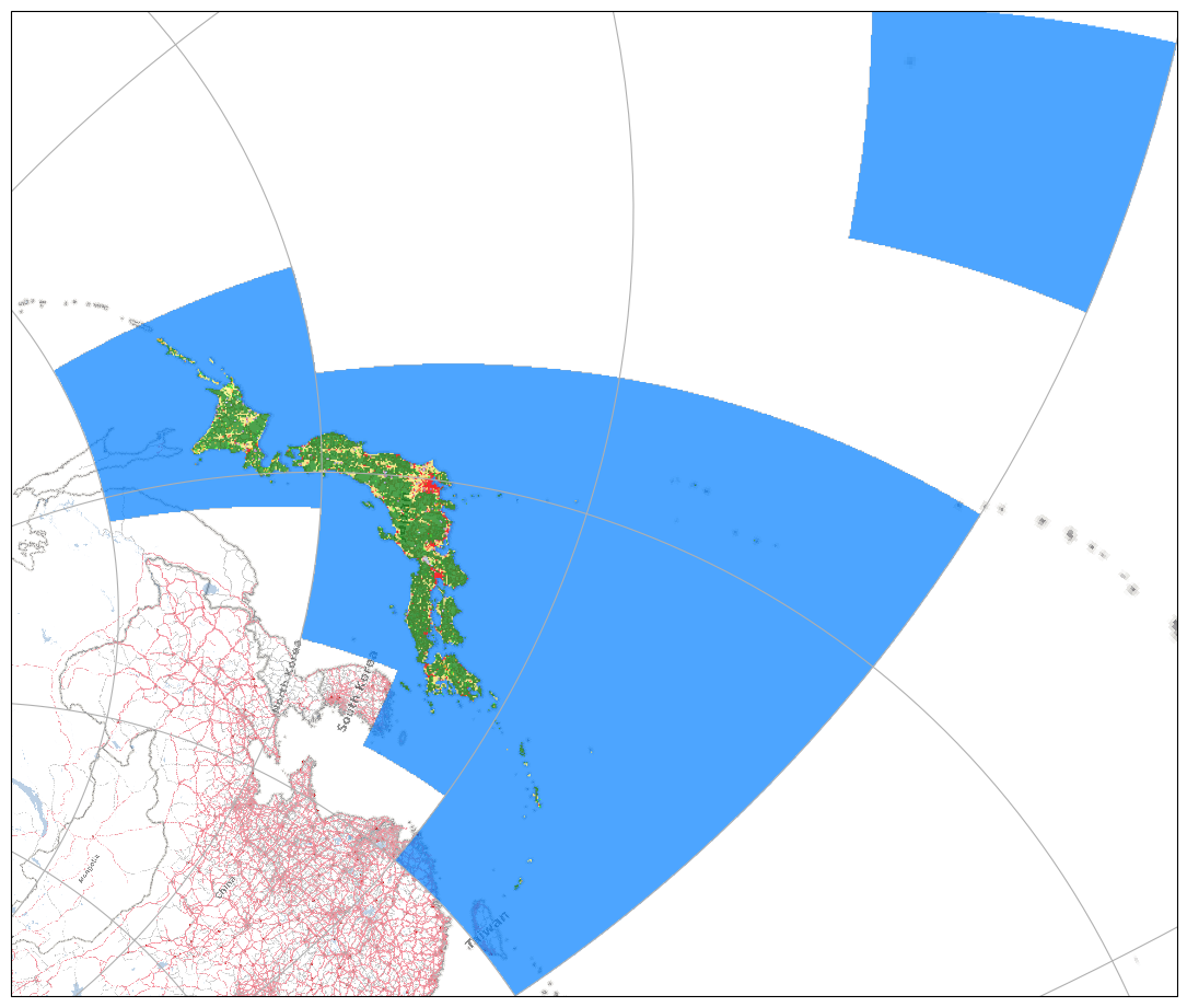
Stereographic してみてるのは単なるお遊び。layer を変えたのが本質なのかも。
zorderをコントロールしないと透けないパターンも見つけた:
 1 # -*- coding: utf-8 -*-
 2 from PIL import Image
 3 import numpy as np
 4 import matplotlib.pyplot as plt
 5 import cartopy.crs as ccrs
 6 import cartopy.feature as cfeature
 7 from cartopy.io.img_tiles import Stamen, GoogleTiles
 8 import tifffile
 9
10
11 def getgeotiffdata(img):
12     return tifffile.TiffFile(img).pages[0].geotiff_tags, Image.open(img).size
13
14
15 def gettransforms(geotiffdata):
16     """
17     build modeltransformation from modelpixelscale, and modeltiepoint
18     """
19     transforms = []
20     if "ModelPixelScale" in geotiffdata and "ModelTiepoint" in geotiffdata:
21         # see "B.6. GeoTIFF Tags for Coordinate Transformations"
22         # in https://earthdata.nasa.gov/files/19-008r4.pdf.
23         sx, sy, sz = geotiffdata["ModelPixelScale"]
24         tiepoints = geotiffdata["ModelTiepoint"]
25         for tp in range(0, len(tiepoints), 6):
26             i, j, k, x, y, z = tiepoints[tp:tp + 6]
27             transforms.append([
28                 [sx, 0.0, 0.0, x - i * sx],
29                 [0.0, -sy, 0.0, y + j * sy],
30                 [0.0, 0.0, sz, z - k * sz],
31                 [0.0, 0.0, 0.0, 1.0]])
32     return transforms
33
34
35 def main():
36     # 国土地理院配布の地勢図
37     # see "Geospatial Information Authority of Japan Website Terms of Use",
38     # http://www.gsi.go.jp/ENGLISH/page_e30286.html
39     geotiffdata, (width, height) = getgeotiffdata(
40         "gm-jpn-lu_u_1_1/jpn/lu.tif")
41     #
42     #print(geotiffdata)
43     transforms = gettransforms(geotiffdata)
44     bb_tl = np.dot(transforms, [0, 0, 0, 1])[0, :2]  # top-left
45     bb_br = np.dot(transforms, [width, height, 0, 1])[0, :2]  # bottom-right
46     #
47     fig = plt.figure()
48     fig.set_size_inches(16.53, 11.69)
49     #crs = ccrs.Stereographic(
50     #    (bb_br[1] + bb_tl[1]) / 2, (bb_br[0] + bb_tl[0]) / 2)
51     crs = ccrs.Stereographic()
52     tiler = GoogleTiles(style="satellite")
53     ax1 = fig.add_subplot(projection=crs)
54     ax1.set_extent(
55         [bb_tl[0], bb_br[0], bb_br[1], bb_tl[1]],
56         ccrs.PlateCarree())
57     ax1.add_image(tiler, 5)
58     ax1.gridlines()
59     #
60     img = plt.imread("gm-jpn-lu_u_1_1/jpn/lu.tif")[:,:,:3]
61     alpha = np.full((img.shape[0], img.shape[1], 1), int(0.7*255))
62     zeroe = (img == 0)
63     zeroe = np.logical_and(zeroe[:,:,0], zeroe[:,:,1], zeroe[:,:,2])
64     alpha[np.where(zeroe)] = 0
65     img_rgba = np.concatenate((img, alpha), axis=2)
66     ax1.imshow(
67         img_rgba,
68         origin='upper',
69         extent=[bb_tl[0], bb_br[0], bb_br[1], bb_tl[1]],
70         transform=ccrs.PlateCarree(),
71         alpha=np.flipud(alpha.reshape(*alpha.shape[:2])),
72         zorder=9
73     )
74
75     plt.savefig("exam_imshow_04_geoaxis_geotiff_2-4_6.png", bbox_inches="tight")
76     plt.close(fig)
77
78
79 if __name__ == '__main__':
80     main()
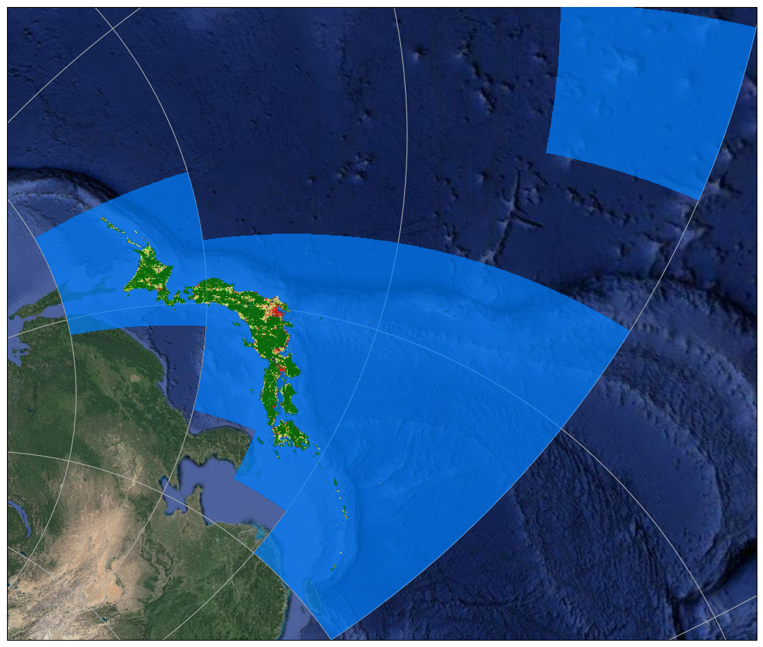
これらのことから、「RGBA を作りそれを imshow に渡すイメージとし、なおかつそのアルファチャンネル部分を imshow の alpha として同時に渡しつつ、なおかつ imshow に渡す zorder も制御する」というのが一番どのパターンでも通用する、という気がする。釈然とはしてないよ、けど、実験結果からするとそういうことになる。
というか…。「もともと RGBA である」のだからこれでいいのでは:
1     # ...
2     ax1.imshow(
3         img,
4         origin='upper',
5         extent=[bb_tl[0], bb_br[0], bb_br[1], bb_tl[1]],
6         transform=ccrs.PlateCarree(),
7         alpha=np.flipud(img[:,:,3].reshape(*img.shape[:2]))
8     )
9     # ...
と言いたかったけれど、「アルファが全部 255 (つまり 1.0)」だったので、意味なかった、これの場合。
よしよし、スケスケ問題はオールクリアだ、と思ったが、そう甘くなかった。「タダで GeoTIFF サンプル欲しいなぁ」と Remote Pixel に辿り着いてみることが出来るのだけれど、たとえばこれは 16bit grayscale なのよね。だから上でやったような alpha の扱いと同じには出来なくて。ひとまずたとえば:
 1 # -*- coding: utf-8 -*-
 2 from PIL import Image
 3 import numpy as np
 4 import matplotlib.pyplot as plt
 5 import cartopy.crs as ccrs
 6 import cartopy.feature as cfeature
 7 import tifffile
 8
 9
10 def getgeotiffdata(img):
11     return tifffile.TiffFile(img).pages[0].geotiff_tags, Image.open(img).size
12
13
14 def gettransforms(geotiffdata):
15     """
16     build modeltransformation from modelpixelscale, and modeltiepoint
17     """
18     transforms = []
19     if "ModelPixelScale" in geotiffdata and "ModelTiepoint" in geotiffdata:
20         # see "B.6. GeoTIFF Tags for Coordinate Transformations"
21         # in https://earthdata.nasa.gov/files/19-008r4.pdf.
22         sx, sy, sz = geotiffdata["ModelPixelScale"]
23         tiepoints = geotiffdata["ModelTiepoint"]
24         for tp in range(0, len(tiepoints), 6):
25             i, j, k, x, y, z = tiepoints[tp:tp + 6]
26             transforms.append([
27                 [sx, 0.0, 0.0, x - i * sx],
28                 [0.0, -sy, 0.0, y + j * sy],
29                 [0.0, 0.0, sz, z - k * sz],
30                 [0.0, 0.0, 0.0, 1.0]])
31     return transforms
32
33
34 def main():
35     geotiffdata, (width, height) = getgeotiffdata(
36         "LC08_L1GT_013032_20210429_20210429_01_RT_B11.tif")
37     #
38     transforms = gettransforms(geotiffdata)
39     bb_tl = np.dot(transforms, [0, 0, 0, 1])[0, :2]  # top-left
40     bb_br = np.dot(transforms, [width, height, 0, 1])[0, :2]  # bottom-right
41     #
42     fig = plt.figure()
43     fig.set_size_inches(16.53, 11.69)
44     crs = ccrs.UTM("18N")
45     ax1 = fig.add_subplot(projection=crs)
46     ext_outer = [
47         bb_tl[0], bb_br[0],
48         bb_br[1], bb_tl[1]]
49     ext_inner = [bb_tl[0], bb_br[0], bb_br[1], bb_tl[1]]
50     ax1.set_extent(ext_outer, crs)
51     #
52     ax1.coastlines(resolution="10m")
53     ax1.gridlines()
54     ax1.add_feature(cfeature.OCEAN, alpha=0.5)
55     ax1.add_feature(cfeature.LAND, alpha=0.5)
56     img = plt.imread("LC08_L1GT_013032_20210429_20210429_01_RT_B11.tif")
57     #
58     alpha = np.full((img.shape[0], img.shape[1]), 1, dtype=np.uint8)
59     alpha[np.where(img == 0)] = 0
60     #
61     ax1.imshow(
62         img,
63         origin='upper',
64         extent=ext_inner,
65         transform=crs, cmap="gray",
66         zorder=-1,
67         alpha=alpha,
68     )
69     plt.savefig(
70         "exam_imshow_04_geoaxis_geotiff_2-4_9.png",
71         bbox_inches="tight")
72     plt.close(fig)
73
74
75 if __name__ == '__main__':
76     main()
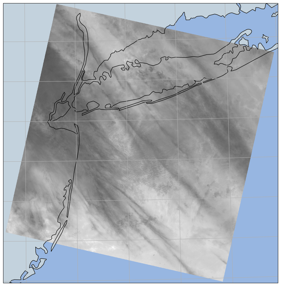
テクニカルには「(width, height, (R, G, B, A))形式に変換」して処理すれば、上でやったやり方と同じに出来ることにはなるのだが、画像サイズが非常にデカいために、よほどのモンスターマシンでない限りは、とんでもなく時間がかかる。たぶん時間がかかってるのはアロケート。ゆえに高速に処理を済ませたければここでやったようにするしかないのだが、ところがこのやり方だと、アルファ値として 0 と 1 しか選べない。dtype=np.uint8 でなければならないのに 0~1 でなければならない、という2つの制約を突きつけられるから。なかなかに弱った状態である。
処理時間を問わないのであれば、「(width, height, (R, G, B, A))形式に変換」するのがいいと思う。ただし、この場合は入口が matplotlib.imread ではなくて、PIL.Image.open になる。この Image オブジェクトの convert メソッドで RGB(A) に変換し、getdata で numpy.ndarray にして…という流れ。だけどね、「3秒で終わる処理が、10分かかるようになる」というほどにヒドい処理時間増加なので、そこはご覚悟を。
ほとんどオマケの話。
ここまでは「ラスタ画像そのものが目的のもので、それを地図背景の上に描画する」というタイプの使い方で、例えば空港の aerodrome chart とどうにか緯度経度を紐付けて地図上に重ねたい、みたいなことをしたい場合に使う使い方ね。一方で、「ラスタ画像を背景として使いたい」というのもあるはず。こちらは、GoogleTiles を始めとするかなり情報量豊富な地図サーバが使えるという理由により、今やあまり必要とされなくなってるんじゃないかという気がする。もともとは上で例にしてた「landsat」なんてのがまさしく「背景画として使いたい」ものだったはずなんだよね、けれども今や「背景画として使いたい」だけなら素直に GoogleTiles などを使えばいい、利用規約の問題がないのであれば。それでもなおやりたいのだ、として。
OpenStreetMap からジオメトリ取得するこのネタも活用して:
  1 # -*- coding: utf-8 -*-
  2 import io
  3 import os
  4 import hashlib
  5 import tempfile
  6 import urllib.request
  7 from collections import namedtuple
  8 import xml.etree.ElementTree as ET
  9 from PIL import Image
 10 import numpy as np
 11 import shapely.wkt
 12 import matplotlib.pyplot as plt
 13 import cartopy.crs as ccrs
 14 import cartopy.feature as cfeature
 15 import tifffile
 16 from shapely.geometry import asPolygon, asLineString
 17
 18
 19 def getgeotiffdata(img):
 20     return tifffile.TiffFile(img).pages[0].geotiff_tags, Image.open(img).size
 21
 22
 23 def gettransforms(geotiffdata):
 24     """
 25     build modeltransformation from modelpixelscale, and modeltiepoint
 26     """
 27     transforms = []
 28     if "ModelPixelScale" in geotiffdata and "ModelTiepoint" in geotiffdata:
 29         # see "B.6. GeoTIFF Tags for Coordinate Transformations"
 30         # in https://earthdata.nasa.gov/files/19-008r4.pdf.
 31         sx, sy, sz = geotiffdata["ModelPixelScale"]
 32         tiepoints = geotiffdata["ModelTiepoint"]
 33         for tp in range(0, len(tiepoints), 6):
 34             i, j, k, x, y, z = tiepoints[tp:tp + 6]
 35             transforms.append([
 36                 [sx, 0.0, 0.0, x - i * sx],
 37                 [0.0, -sy, 0.0, y + j * sy],
 38                 [0.0, 0.0, sz, z - k * sz],
 39                 [0.0, 0.0, 0.0, 1.0]])
 40     return transforms
 41
 42
 43 def osmquery(args):
 44     _BASEURI = "http://www.overpass-api.de/api/xapi?"
 45     clon, clat, width = args.clon, args.clat, args.width
 46     degpermetre = 1 / (30.0 * 3600)
 47     ext = (width / 2) * degpermetre
 48     bbox = (clon - ext, clat - ext, clon + ext, clat + ext)
 49     fq = ""
 50     if args.feature_query:
 51         fq = "[{}]".format(urllib.request.quote(args.feature_query))
 52     uri = _BASEURI + "*{fq}[bbox={bb}]".format(
 53         fq=fq, bb=",".join(["{:.4f}".format(p) for p in bbox]))
 54     resf = os.path.join(
 55         tempfile.gettempdir(),
 56         "xapi_" + hashlib.md5(uri.encode("utf-8")).hexdigest())
 57     if not os.path.exists(resf):
 58         cont, msg = urllib.request.urlretrieve(uri)
 59         os.rename(cont, resf)
 60     parsed = ET.parse(resf)
 61     nodes = {}  # id: (lon, lat)
 62     ways = {}
 63     for tle in parsed.getroot():
 64         if tle.tag == "node":
 65             id = tle.attrib["id"]
 66             lon = float(tle.attrib["lon"])
 67             lat = float(tle.attrib["lat"])
 68             nodes[id] = (lon, lat)
 69     for tle in parsed.getroot():
 70         if tle.tag == "way":
 71             thisway = {}
 72             pts = []
 73             for che in tle:
 74                 if che.tag == "nd":
 75                     refid = che.attrib["ref"]
 76                     pts.append(nodes[refid])
 77                 elif che.tag == "tag":
 78                     thisway[che.attrib["k"]] = che.attrib["v"]
 79             if pts[0] == pts[-1]:
 80                 poly = asPolygon(pts)
 81             else:
 82                 poly = asLineString(pts)
 83             try:  # check if valid polygon
 84                 poly.type  # cause Exception from shapely if it is not valid
 85                 thisway["geometry"] = poly
 86                 ways[tle.attrib["id"]] = thisway
 87             except ValueError:
 88                 pass
 89     return ways
 90
 91
 92 def main():
 93     # Kelsey Jordahl (Enthought)'s DATA_CREDITS.md says:
 94     #     The file `manhattan.tif` is a [Digital Orthophoto Quadrangle (DOQ)]
 95     #     (https://lta.cr.usgs.gov/DOQs) from the USGS and in the public domain
 96     #     ([direct link](http://earthexplorer.usgs.gov/metadata/1131/DI00000000845784)).
 97     #     They [request](https://lta.cr.usgs.gov/citation) the following attribution
 98     #     statement when using thir data:
 99     #     "Data available from the U.S. Geological Survey."
100     geotiffdata, (width, height) = getgeotiffdata(
101         "data/manhattan.tif")
102     #
103     transforms = gettransforms(geotiffdata)
104     bb_tl = np.dot(transforms, [0, 0, 0, 1])[0,:2]  # top-left
105     bb_br = np.dot(transforms, [width, height, 0, 1])[0,:2]  # bottom-right
106     #
107     fig = plt.figure()
108     fig.set_size_inches(16.53, 11.69)
109     crs = ccrs.UTM("18N")
110     ax1 = fig.add_subplot(projection=crs)
111     ax1.set_extent(
112         [bb_tl[0] - 10**3, bb_br[0] + 2 * 10**3, bb_br[1] - 10**3, bb_tl[1] + 10**3],
113         crs)
114     #
115     img = plt.imread("data/manhattan.tif")
116     ax1.imshow(
117         img,
118         origin='upper',
119         extent=[bb_tl[0], bb_br[0], bb_br[1], bb_tl[1]],
120         transform=crs)
121     #
122     QArg = namedtuple('QArg', ['clon', 'clat', 'width', 'feature_query'])
123     ways_park = {}
124     ways_park.update(
125         osmquery(QArg(-73.9559, 40.7788, 10000, 'name=Central Park')))
126     ways_park.update(
127         osmquery(QArg(-73.9559, 40.7788, 10000, 'name=Riverside Park')))
128     ways_park.update(
129         osmquery(QArg(-73.9559, 40.7788, 10000, 'name=Riverbank State Park')))
130     ways_park.update(
131         osmquery(QArg(-73.9559, 40.7788, 10000, 'name=Wards Island Park')))
132     ways_park.update(
133         osmquery(QArg(-73.9559, 40.7788, 10000, 'name=North Hudson Park')))
134     ways_park.update(
135         osmquery(QArg(-73.9559, 40.7788, 10000, 'name=Randalls Island Park')))
136     ax1.add_geometries(
137         [v["geometry"] for k, v in ways_park.items()],
138         ccrs.PlateCarree(),
139         facecolor='#00ff0011', edgecolor='#0000ff', linewidth=3)
140     ways_build = {}
141     ways_build.update(
142         osmquery(QArg(-73.9559, 40.7788, 10000, 'public_transport=*')))
143     ax1.add_geometries(
144         [v["geometry"] for k, v in ways_build.items()],
145         ccrs.PlateCarree(),
146         facecolor='#ffff0099', edgecolor='#000000', linewidth=0.1)
147     ways_railway = {}
148     ways_railway.update(
149         osmquery(QArg(-73.9559, 40.7788, 10000, 'railway=*')))
150     for k, v in ways_railway.items():
151         if v["geometry"].geom_type == "Polygon":
152             ax1.add_geometries(
153                 [v["geometry"]],
154                 ccrs.PlateCarree(),
155                 facecolor='#00ffff10', edgecolor='black', linewidth=0.1)
156         else:
157             ax1.add_geometries(
158                 [v["geometry"]],
159                 ccrs.PlateCarree(),
160                 facecolor='none', edgecolor='black', linewidth=0.2)
161     ax1.set_title("Data available from the U.S. Geological Survey.")
162     plt.savefig("exam_imshow_04_geoaxis_geotiff_2-4_7____.png", bbox_inches="tight")
163     plt.close(fig)
164
165
166 if __name__ == '__main__':
167     main()
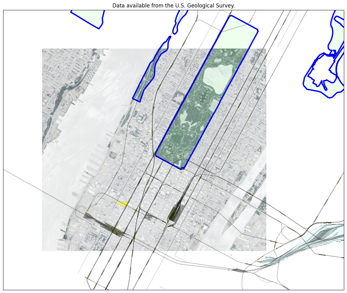
ここでは add_geometries したが、当たり前だが「観測データの行列を pcolor する」だのあれやこれや、てのは、話としてはまさしく(3)~に戻るだけの話。ただ、「文字を書く」のをやってみて、(5)では気付かなかった問題がわかった:
  1 # -*- coding: utf-8 -*-
  2 import io
  3 import os
  4 import hashlib
  5 import tempfile
  6 import urllib.request
  7 from collections import namedtuple
  8 import xml.etree.ElementTree as ET
  9 from PIL import Image
 10 import numpy as np
 11 import shapely.geometry as sgeom
 12 import shapely.wkt
 13 import matplotlib.pyplot as plt
 14 from matplotlib.transforms import offset_copy
 15 import cartopy.crs as ccrs
 16 import cartopy.feature as cfeature
 17 import tifffile
 18 from shapely.geometry import asPolygon, asLineString
 19
 20
 21 def getgeotiffdata(img):
 22     return tifffile.TiffFile(img).pages[0].geotiff_tags, Image.open(img).size
 23
 24
 25 def gettransforms(geotiffdata):
 26     """
 27     build modeltransformation from modelpixelscale, and modeltiepoint
 28     """
 29     transforms = []
 30     if "ModelPixelScale" in geotiffdata and "ModelTiepoint" in geotiffdata:
 31         # see "B.6. GeoTIFF Tags for Coordinate Transformations"
 32         # in https://earthdata.nasa.gov/files/19-008r4.pdf.
 33         sx, sy, sz = geotiffdata["ModelPixelScale"]
 34         tiepoints = geotiffdata["ModelTiepoint"]
 35         for tp in range(0, len(tiepoints), 6):
 36             i, j, k, x, y, z = tiepoints[tp:tp + 6]
 37             transforms.append([
 38                 [sx, 0.0, 0.0, x - i * sx],
 39                 [0.0, -sy, 0.0, y + j * sy],
 40                 [0.0, 0.0, sz, z - k * sz],
 41                 [0.0, 0.0, 0.0, 1.0]])
 42     return transforms
 43
 44
 45 def osmquery(args):
 46     _BASEURI = "http://www.overpass-api.de/api/xapi?"
 47     clon, clat, width = args.clon, args.clat, args.width
 48     degpermetre = 1 / (30.0 * 3600)
 49     ext = (width / 2) * degpermetre
 50     bbox = (clon - ext, clat - ext, clon + ext, clat + ext)
 51     fq = ""
 52     if args.feature_query:
 53         fq = "[{}]".format(urllib.request.quote(args.feature_query))
 54     uri = _BASEURI + "*{fq}[bbox={bb}]".format(
 55         fq=fq, bb=",".join(["{:.4f}".format(p) for p in bbox]))
 56     resf = os.path.join(
 57         tempfile.gettempdir(),
 58         "xapi_" + hashlib.md5(uri.encode("utf-8")).hexdigest())
 59     if not os.path.exists(resf):
 60         cont, msg = urllib.request.urlretrieve(uri)
 61         os.rename(cont, resf)
 62     parsed = ET.parse(resf)
 63     nodes = {}  # id: (lon, lat)
 64     ways = {}
 65     for tle in parsed.getroot():
 66         if tle.tag == "node":
 67             id = tle.attrib["id"]
 68             lon = float(tle.attrib["lon"])
 69             lat = float(tle.attrib["lat"])
 70             nodes[id] = (lon, lat)
 71     for tle in parsed.getroot():
 72         if tle.tag == "way":
 73             thisway = {}
 74             pts = []
 75             for che in tle:
 76                 if che.tag == "nd":
 77                     refid = che.attrib["ref"]
 78                     pts.append(nodes[refid])
 79                 elif che.tag == "tag":
 80                     thisway[che.attrib["k"]] = che.attrib["v"]
 81             if pts[0] == pts[-1]:
 82                 poly = asPolygon(pts)
 83             else:
 84                 poly = asLineString(pts)
 85             try:  # check if valid polygon
 86                 poly.type  # cause Exception from shapely if it is not valid
 87                 thisway["geometry"] = poly
 88                 ways[tle.attrib["id"]] = thisway
 89             except ValueError:
 90                 pass
 91     return ways
 92
 93
 94 def main():
 95     # Kelsey Jordahl (Enthought)'s DATA_CREDITS.md says:
 96     #     The file `manhattan.tif` is a [Digital Orthophoto Quadrangle (DOQ)]
 97     #     (https://lta.cr.usgs.gov/DOQs) from the USGS and in the public domain
 98     #     ([direct link](http://earthexplorer.usgs.gov/metadata/1131/DI00000000845784)).
 99     #     They [request](https://lta.cr.usgs.gov/citation) the following attribution
100     #     statement when using thir data:
101     #     "Data available from the U.S. Geological Survey."
102     geotiffdata, (width, height) = getgeotiffdata(
103         "data/manhattan.tif")
104     #
105     transforms = gettransforms(geotiffdata)
106     bb_tl = np.dot(transforms, [0, 0, 0, 1])[0,:2]  # top-left
107     bb_br = np.dot(transforms, [width, height, 0, 1])[0,:2]  # bottom-right
108     #
109     fig = plt.figure()
110     fig.set_size_inches(16.53, 11.69)
111     crs = ccrs.UTM("18N")
112     ax1 = fig.add_subplot(projection=crs)
113     ext_outer = [
114         bb_tl[0] - 0.5 * 10**3, bb_br[0] + 2.5 * 10**3,
115         bb_br[1] - 0.5 * 10**3, bb_tl[1] + 2.5 * 10**3]
116     ext_inner = [bb_tl[0], bb_br[0], bb_br[1], bb_tl[1]]
117     ax1.set_extent(ext_outer, crs)
118     #
119     img = plt.imread("data/manhattan.tif")
120     ax1.imshow(
121         img,
122         origin='upper',
123         extent=ext_inner,
124         transform=crs)
125     #
126     geodetic_transform = ccrs.Geodetic()._as_mpl_transform(ax1)
127     text_transform = offset_copy(geodetic_transform, units='dots', x=2)
128     #
129     QArg = namedtuple('QArg', ['clon', 'clat', 'width', 'feature_query'])
130     ways_park = {}
131     ways_park.update(
132         osmquery(QArg(-73.9559, 40.7788, 10000, 'name=Central Park')))
133     ways_park.update(
134         osmquery(QArg(-73.9559, 40.7788, 10000, 'name=Riverside Park')))
135     ways_park.update(
136         osmquery(QArg(-73.9559, 40.7788, 10000, 'name=Riverbank State Park')))
137     ways_park.update(
138         osmquery(QArg(-73.9559, 40.7788, 10000, 'name=Wards Island Park')))
139     ways_park.update(
140         osmquery(QArg(-73.9559, 40.7788, 10000, 'name=North Hudson Park')))
141     ways_park.update(
142         osmquery(QArg(-73.9559, 40.7788, 10000, 'name=Randalls Island Park')))
143     ax1.add_geometries(
144         [v["geometry"] for k, v in ways_park.items()],
145         ccrs.PlateCarree(),
146         facecolor='#00ff0011', edgecolor='#0000ff', linewidth=3)
147     #
148     ext_outer = sgeom.box(*ext_outer)
149     for k, v in ways_park.items():
150         if v.get("name"):
151             ct = v["geometry"].centroid
152             if crs.project_geometry(ct, ccrs.PlateCarree()).within(ext_outer):
153                 ax1.text(ct.x, ct.y, "{}".format(v["name"]),
154                          verticalalignment='center', horizontalalignment='right',
155                          transform=text_transform,
156                          fontproperties=dict(family="Comic Sans MS", size=18),
157                          color="blue",
158                          #bbox=dict(facecolor='green', alpha=0.5, boxstyle='round')
159                          )
160     #
161     ways_build = {}
162     ways_build.update(
163         osmquery(QArg(-73.9559, 40.7788, 10000, 'public_transport=*')))
164     ax1.add_geometries(
165         [v["geometry"] for k, v in ways_build.items()],
166         ccrs.PlateCarree(),
167         facecolor='#ffff0099', edgecolor='#000000', linewidth=0.1)
168     ways_railway = {}
169     ways_railway.update(
170         osmquery(QArg(-73.9559, 40.7788, 10000, 'railway=*')))
171     for k, v in ways_railway.items():
172         if v["geometry"].geom_type == "Polygon":
173             ax1.add_geometries(
174                 [v["geometry"]],
175                 ccrs.PlateCarree(),
176                 facecolor='#00ffff10', edgecolor='black', linewidth=0.1)
177         else:
178             ax1.add_geometries(
179                 [v["geometry"]],
180                 ccrs.PlateCarree(),
181                 facecolor='none', edgecolor='black', linewidth=0.2)
182     ax1.set_title("Data available from the U.S. Geological Survey.")
183     plt.savefig(
184         "exam_imshow_04_geoaxis_geotiff_2-4_8__.png", bbox_inches="tight")
185     plt.close(fig)
186
187
188 if __name__ == '__main__':
189     main()
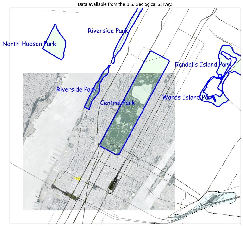
そもそも、「画像とグリッドデータと地図の重ね合わせ」というニーズというのは、「仮想と現実のマッピングをしたいから」というところから発生していることが多い。観測データや予測データが、「位置に結び付けなければこれはただの行列データ」の場合に、機械のためには行列データの行・列と経度・緯度(などの位置情報)と結びつけるだけで十分である。「絵としての地図」にまで結びつけたいのはこれは人間のためであって、すなわち、「この気温予測グリッドデータの (i, j) = (23, 42) というのは、一体全体東京都のどこなんだい?」ということを、人間が目で見て知りたい、ということ。上で例にした LC08_L1GT_013032_20210429_20210429_01_RT_B11.tif についても、これは画像としては雲量だけが含まれていて、「どこの雲やねん」というのを人間が知るためには、やはり地図と重ねたい、てわけだ。
して、LC08_L1GT_013032_20210429_20210429_01_RT_B11.tif については、先に苦労したように、透かすのが難儀で、なので、有効データ範囲内については WMS や GoogleTiles と重ねて使うのがキビシイ。これの場合は範囲もとても大きいため、海岸線描画だけだと今ひとつ位置の把握がしづらく、何か補助情報を描画したい、という気分になるわけだ。つまり「地図上にテキストを描画したい」。空港の位置だけでも、てのがひとまず良いかもなぁと:
  1 # -*- coding: utf-8 -*-
  2 import os
  3 import hashlib
  4 import tempfile
  5 import urllib.request
  6 from collections import namedtuple
  7 import xml.etree.ElementTree as ET
  8 from PIL import Image
  9 import numpy as np
 10 import matplotlib.pyplot as plt
 11 from matplotlib.transforms import offset_copy
 12 import cartopy.crs as ccrs
 13 import cartopy.feature as cfeature
 14 import tifffile
 15 from shapely.geometry import asPolygon, asLineString
 16 import shapely.geometry as sgeom
 17 from pyproj import Transformer
 18
 19
 20 def getgeotiffdata(img):
 21     return tifffile.TiffFile(img).pages[0].geotiff_tags, Image.open(img).size
 22
 23
 24 def gettransforms(geotiffdata):
 25     """
 26     build modeltransformation from modelpixelscale, and modeltiepoint
 27     """
 28     transforms = []
 29     if "ModelPixelScale" in geotiffdata and "ModelTiepoint" in geotiffdata:
 30         # see "B.6. GeoTIFF Tags for Coordinate Transformations"
 31         # in https://earthdata.nasa.gov/files/19-008r4.pdf.
 32         sx, sy, sz = geotiffdata["ModelPixelScale"]
 33         tiepoints = geotiffdata["ModelTiepoint"]
 34         for tp in range(0, len(tiepoints), 6):
 35             i, j, k, x, y, z = tiepoints[tp:tp + 6]
 36             transforms.append([
 37                 [sx, 0.0, 0.0, x - i * sx],
 38                 [0.0, -sy, 0.0, y + j * sy],
 39                 [0.0, 0.0, sz, z - k * sz],
 40                 [0.0, 0.0, 0.0, 1.0]])
 41     return transforms
 42
 43
 44 def osmquery(args):
 45     _BASEURI = "http://www.overpass-api.de/api/xapi?"
 46     bbox = args.bbox
 47     fq = ""
 48     if args.feature_query:
 49         fq = "[{}]".format(urllib.request.quote(args.feature_query))
 50     uri = _BASEURI + "*{fq}[bbox={bb}]".format(
 51         fq=fq, bb=",".join(["{:.4f}".format(p) for p in bbox]))
 52     resf = os.path.join(
 53         tempfile.gettempdir(),
 54         "xapi_" + hashlib.md5(uri.encode("utf-8")).hexdigest())
 55     if not os.path.exists(resf):
 56         cont, msg = urllib.request.urlretrieve(uri)
 57         os.rename(cont, resf)
 58     parsed = ET.parse(resf)
 59     nodes = {}  # id: (lon, lat)
 60     ways = {}
 61     for tle in parsed.getroot():
 62         if tle.tag == "node":
 63             id = tle.attrib["id"]
 64             lon = float(tle.attrib["lon"])
 65             lat = float(tle.attrib["lat"])
 66             nodes[id] = (lon, lat)
 67     for tle in parsed.getroot():
 68         if tle.tag == "way":
 69             thisway = {}
 70             pts = []
 71             for che in tle:
 72                 if che.tag == "nd":
 73                     refid = che.attrib["ref"]
 74                     pts.append(nodes[refid])
 75                 elif che.tag == "tag":
 76                     thisway[che.attrib["k"]] = che.attrib["v"]
 77             if pts[0] == pts[-1]:
 78                 poly = asPolygon(pts)
 79             else:
 80                 poly = asLineString(pts)
 81             try:  # check if valid polygon
 82                 poly.type  # cause Exception from shapely if it is not valid
 83                 thisway["geometry"] = poly
 84                 ways[tle.attrib["id"]] = thisway
 85             except ValueError:
 86                 pass
 87     return ways
 88
 89
 90 def main():
 91     utmzone, utmepsg = "18N", 32618
 92     tiffname = "LC08_L1GT_013032_20210429_20210429_01_RT_B11.tif"
 93     #utmzone, utmepsg = "54N", 32654
 94     #tiffname = "LC08_L1TP_107033_20210518_20210518_01_RT_B1.tif"
 95     geotiffdata, (width, height) = getgeotiffdata(
 96         tiffname)
 97     #print(geotiffdata)
 98     #
 99     transforms = gettransforms(geotiffdata)
100     bb_tl = np.dot(transforms, [0, 0, 0, 1])[0, :2]  # top-left
101     bb_br = np.dot(transforms, [width, height, 0, 1])[0, :2]  # bottom-right
102     #
103     fig = plt.figure()
104     fig.set_size_inches(16.53, 11.69)
105     crs = ccrs.UTM(utmzone)
106     ax1 = fig.add_subplot(projection=crs)
107     ext_outer = [
108         bb_tl[0], bb_br[0],
109         bb_br[1], bb_tl[1]]
110     ext_inner = [bb_tl[0], bb_br[0], bb_br[1], bb_tl[1]]
111     ax1.set_extent(ext_outer, crs)
112     #
113     ax1.coastlines(resolution="10m")
114     ax1.gridlines()
115     ax1.add_feature(cfeature.OCEAN, alpha=0.5)
116     ax1.add_feature(cfeature.LAND, alpha=0.5)
117     img = plt.imread(tiffname)
118     #
119     alpha = np.full((img.shape[0], img.shape[1]), 1, dtype=np.uint8)
120     alpha[np.where(img == 0)] = 0
121     #
122     ax1.imshow(
123         img,
124         origin='upper',
125         extent=ext_inner,
126         transform=crs, cmap="gray",
127         zorder=-1,
128         alpha=alpha,
129     )
130     geodetic_transform = ccrs.Geodetic()._as_mpl_transform(ax1)
131     text_transform = offset_copy(geodetic_transform, units='dots', x=96, y=-8)
132     #
133     tr = Transformer.from_crs(utmepsg, 4326)
134     bbbl = tr.transform(*ext_outer[::2])[::-1]
135     bbtr = tr.transform(*ext_outer[1::2])[::-1]
136     bbox = (bbbl[0], bbbl[1], bbtr[0], bbtr[1])
137     QArg = namedtuple('QArg', ['bbox', 'feature_query'])
138     ways = {}
139     ways.update(
140         osmquery(QArg(bbox, 'aeroway=aerodrome')))
141     ext_outer = sgeom.box(*ext_outer)
142     for k, v in ways.items():
143         if v.get("name"):
144             g = v["geometry"]
145             ct = g.centroid
146             # 小さい空港を全部描画すると渋滞した絵になるのである程度大きなものだけ。
147             # area での判定は m^2 単位での正確な判断も出来るが、ラフでいいので
148             # 無次元の値で直接。
149             if g.area > 0.0001 and crs.project_geometry(
150                     ct, ccrs.PlateCarree()).within(ext_outer):
151                 ax1.add_geometries(
152                     [g],
153                     ccrs.PlateCarree(),
154                     facecolor='#ffff0055', edgecolor='#0000ff', linewidth=0.1)
155                 ax1.text(ct.x, ct.y, "{}".format(v.get("name:en", v["name"])),
156                          verticalalignment='center', horizontalalignment='right',
157                          transform=text_transform,
158                          fontproperties=dict(family="Comic Sans MS", size=10),
159                          color="blue",
160                          #bbox=dict(facecolor='green', alpha=0.5, boxstyle='round')
161                          )
162     #print("%f" % np.mean(mm))
163     plt.savefig(
164         "exam_imshow_04_geoaxis_geotiff_2-4_9_2_2.png",
165         bbox_inches="tight")
166     plt.close(fig)
167
168
169 if __name__ == '__main__':
170     main()
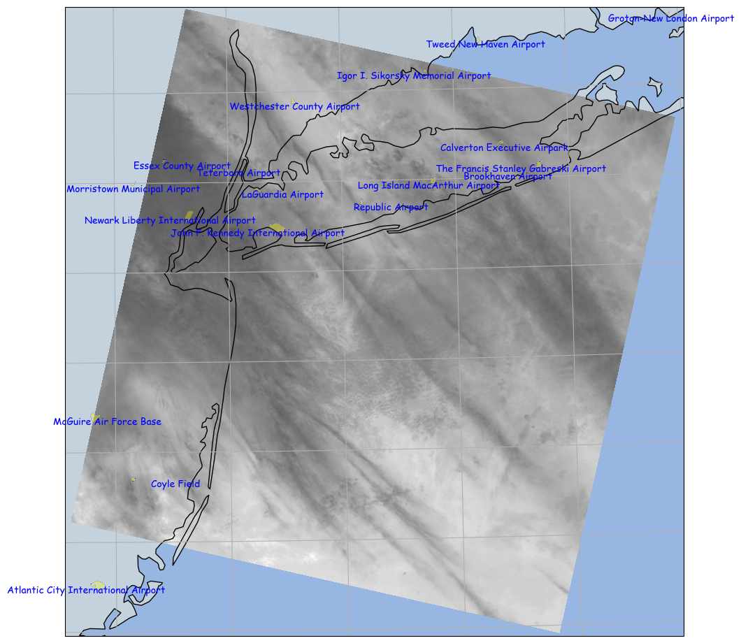
空港の位置がプロットされてるだけで格段にわかりやすいと感じるかどうかなんてのは、まぁ人によるとしか言いようがない。ここいらは工夫のしどころ、てとこだ。この例だと説得力が足りないかもしれないけれど、LC08_L1TP_107033_20210518_20210518_01_RT_B1.tif の方を有効にした結果をみれば、ワタシの言いたいことはよりわかるに違いない:
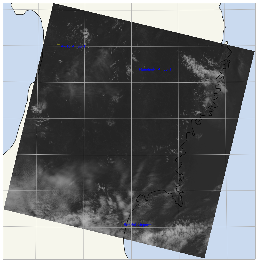
何かしら情報が書かれていないとどこのことやらさっぱりわからんだろう、「Sendai Airport」が描画されてるだけで、随分把握しやすくなると思う。
ところで。
独立したネタとして書くか迷ったんだけれど、一連のスクリプト中ではしれーっとワタシが書いたものでは初出の「cartopy.crs.epsg」を使っているものがある。そこでは geotiff に対する問い合わせで EPSG:3857 であることがわかるので、それを直接使えるから便利だ、てことではあるんだけれど、ただこれ、注意が必要。
cartopy.crs.epsg の実装は、「95.3219876488398713% pyepsg に丸投げ」になっている。そして、pyepsg の実装は、https://epsg.io/ へ丸投げ(たとえば https://epsg.io/3857.gml など参照)。これは言ってしまえば「EPSG データベース」なのだが、それを HTTP GET で毎度お取り寄せるという実現方式を採用している。PROJ なんかがそうであるように、抱え込みで定義データを持つアプローチとは対照的、と言える。
ゆえに、「ワタシの PC とワタシには既知」なものを都度インターネットアクセスしてお取り寄せることの是非、あるいは「未知だったとしても、毎度お尋ねするようなものなのかい?」という疑問に対しては、きちんと自分なりの答えを見つけておくべきだ。少なくとも「いつ何時実行する場合でも同じものを使う」ような、しかもそれが何かの商用目的の製品の実装としてなら、まぁふつうはこれは「アウト」とみなされるのが普通であろう。おそらく Projection 派生の特殊化を自力で書くのが最善で、そうでない場合でも最低でもインターネットアクセスを最小にするべく、キャッシュは検討すべきであろう。
あ、そうそう。pykdtree ね。cartopy が依存しているプロジェクトで、個別に面白いのかしら、と思ったんだよね。R-Tree みたく。
具体的には、この pykdtree、今のところは imshow のみが依存している、と思う。それ以外では今は使われていなそう。ここで regrid_shape のことに触れたが、同じ「regrid_shape」というキー概念に対して、cartopy は複数の実装を与えていて、なぜか imshow 内で使う regrid でだけ pykdtree を使う。
そもそも K-D Tree の実装は、scipy.spatial が既に持っていて、pykdtree をインストールしない場合は、scipy.spatial のものが使われる。ゆえに、scipy ユーザであるワタシにとって、実は目新しいものではないのであった。それと、「初耳」と思ってたら違ってた。前に明示的に調べたことがあった。以下のテストコードを書いてみて思い出したんだよね、「あ、あれか」と:
 1 # -*- coding: utf-8 -*-
 2 import io
 3 import numpy as np
 4 import msgpack
 5 import shapely.wkb
 6 from pykdtree.kdtree import KDTree
 7
 8
 9 def main():
10     # msgpack の形で書き出しておいた都道府県ポリゴン。
11     unpacked = {
12         k: shapely.wkb.loads(v)
13         for k, v in msgpack.unpack(
14                 io.open("polbnda_jpn_prefs.bin", "rb")).items()}
15     #
16     data_pts_real = np.array([list(v.centroid.coords)[0] for k, v in unpacked.items()])
17     tree = KDTree(data_pts_real)
18     targ = [133.3, 33.4]
19     dist, idx = tree.query(np.array([targ]))
20     for i in range(len(idx)):
21         found = data_pts_real[idx[i]]
22         my_dist = (targ[0] - found[0], targ[1] - found[1])
23         my_dist = np.sqrt(my_dist[0]**2 + my_dist[1]**2)
24         print(targ, list(found), my_dist, dist[i])
25
26 if __name__ == '__main__':
27     main()
「distance を自分で計算してみたものと一致するのかしら」と思ったところで記憶が完全によみがえった。
最初、何も思い出す前は、いわゆる位置情報インデクス、まさに R-Tree と同じ役割が期待されて使われてるんだと思ったんだよね。けれども少なくとも cartopy のこれへの依存は、K-D Tree の本来のユースケースの「最近傍探索」のために使ってるだけなんだよね。まぁわかってしまえばそりゃそーか、てことなんだけれども。
てわけで、「今日のオレ」には別にオイシイものではなかった。「明日のワタクシメ」には役に立つかもしらんけどね。