(1)、(2)が、ほぼ導入そのものについてだけだったので、そろそろ「らしいことを」と。
quiver が扱う可視化ってね、「やってみるまで難しさに気付けない」やつだったりすんのよね。地図スケールに関係ない、実験室サイズの実験結果可視化の quiver は別よ、そうじゃなくて、「風速風向予測を日本地図に乗せる」ことは、まさに「スケール」の問題があって、初めてやってみると高確率でつまづく。わかる? 「日本地図」のスケールはたとえば「1ピクセルが500m」というスケールに対して、「u成分が 1m/s、v成分が-0.2m/s」を描画しようとする問題なのだ。「風速」のようなスカラー量、たとえば「20m/s」とかを pcolor とかで描くのにはまったく苦労しないので、始める前はこの難しさについて、なかなか想像出来ないんだよね。違いは「z成分の描画」なのか、「x-y 平面に x, y として描くのか」の違いね。(x-y 平面に描く z は x, y のスケールと z のスケールがどんなに乖離してても全然問題ない。)
てわけで regrid_shape、便利ね:
 1 # -*- coding: utf-8 -*-
 2 import os
 3 import sys
 4 import pygrib
 5 import numpy as np
 6 import cartopy.crs as ccrs
 7 import cartopy.feature as cfeature
 8 from cartopy.mpl.ticker import LongitudeFormatter, LatitudeFormatter
 9 import matplotlib.pyplot as plt
10
11
12 def _read(srcfn):
13     src = pygrib.open(srcfn)
14     for s in src:
15         yield s.level, (s.name, s.parameterName), s.validDate, s.latlons(), s.values
16     src.close()
17
18
19 def main(gpv):
20     key_u, key_v = "U component of wind", "V component of wind"
21     data = {}
22     inivd, inilev = None, None
23     for level, yk, vd, latlons, values in _read(gpv):
24         if key_u in yk and key_u not in data:
25             data[key_u] = latlons, values
26             if inivd is None:
27                 inivd, inilev = vd, level
28         if key_v in yk and key_v not in data:
29             data[key_v] = latlons, values
30             if inivd is None:
31                 inivd, inilev = vd, level
32         if len(data) == 2:
33             break
34     (lats, lons), values_u = data[key_u]
35     _, values_v = data[key_v]
36     X, Y = lons[0,:], lats[:,0]
37     #
38     fig = plt.figure()
39     fig.set_size_inches(16.53, 11.69)
40     crs = ccrs.Geostationary(X.mean())
41     ax1 = fig.add_subplot(projection=crs)
42     ext = [X.min() + 7, X.max() - 5, Y.min() + 5, Y.max() - 2]
43     ax1.set_extent(ext, ccrs.PlateCarree())
44     CS = ax1.pcolormesh(
45         X, Y,
46         np.sqrt(values_u**2 + values_v**2),
47         transform=ccrs.PlateCarree(), shading="auto")
48     rs = (int((ext[1] - ext[0]) * 2), int((ext[3] - ext[2]) * 2))
49     ax1.quiver(
50         X, Y,
51         values_u, values_v,
52         transform=ccrs.PlateCarree(),
53         regrid_shape=rs)
54     ax1.coastlines(resolution="10m")
55     ax1.gridlines()
56     plt.colorbar(CS, ax=ax1)
57     #ax1.add_feature(cfeature.OCEAN)
58     #ax1.add_feature(cfeature.LAND)
59
60     plt.savefig("{}_{}_p{}_{}.png".format(
61         os.path.basename(gpv), str(inivd).partition(":")[0], inilev, "wind"),
62         bbox_inches="tight")
63     #plt.show()
64
65
66 if __name__ == '__main__':
67     # 入力は "Z__C_RJTD_20210514000000_MSM_GPV_Rjp_L-pall_FH00-15_grib2.bin" など。
68     main(sys.argv[1])
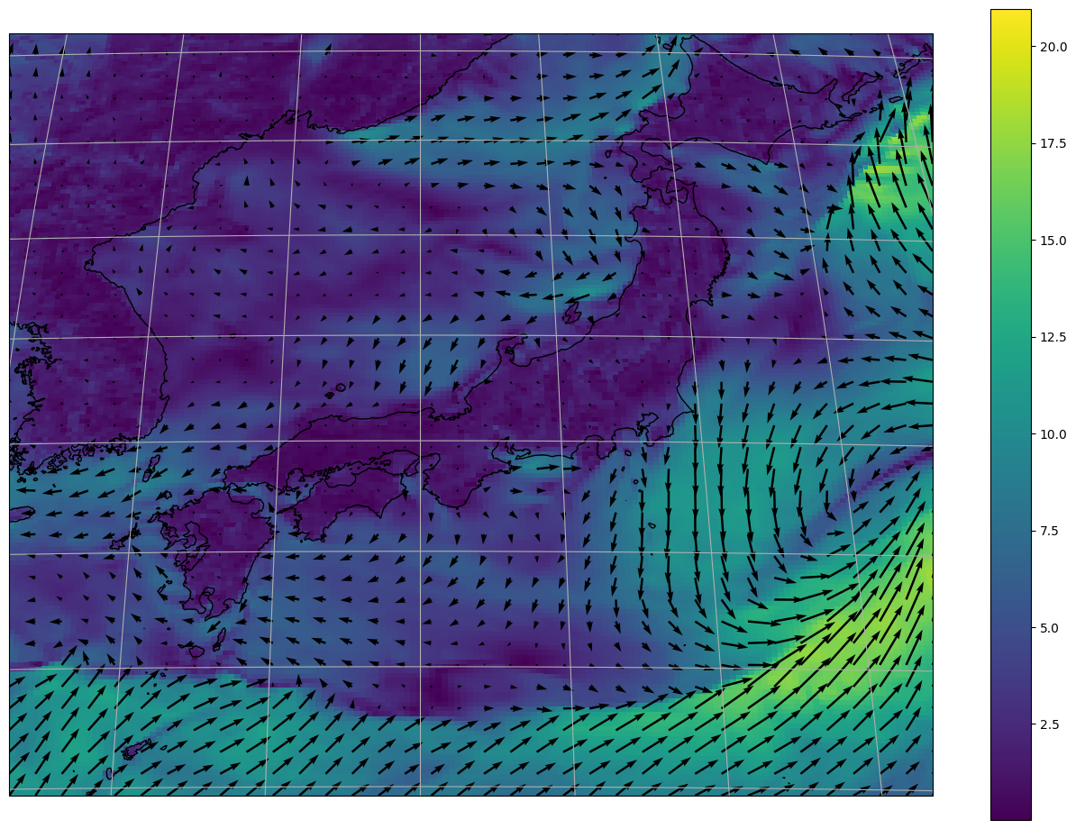
是非 regrid_shape 制御なしの失敗作もご自分でやってみて欲しい。(ワタシは regrid_shape をちょっと細かくコントロールしてるが、意味がつかみにくいなら「regrid_shape=2」「regrid_shape=10」と順に試せば即座に理解できるはず。)
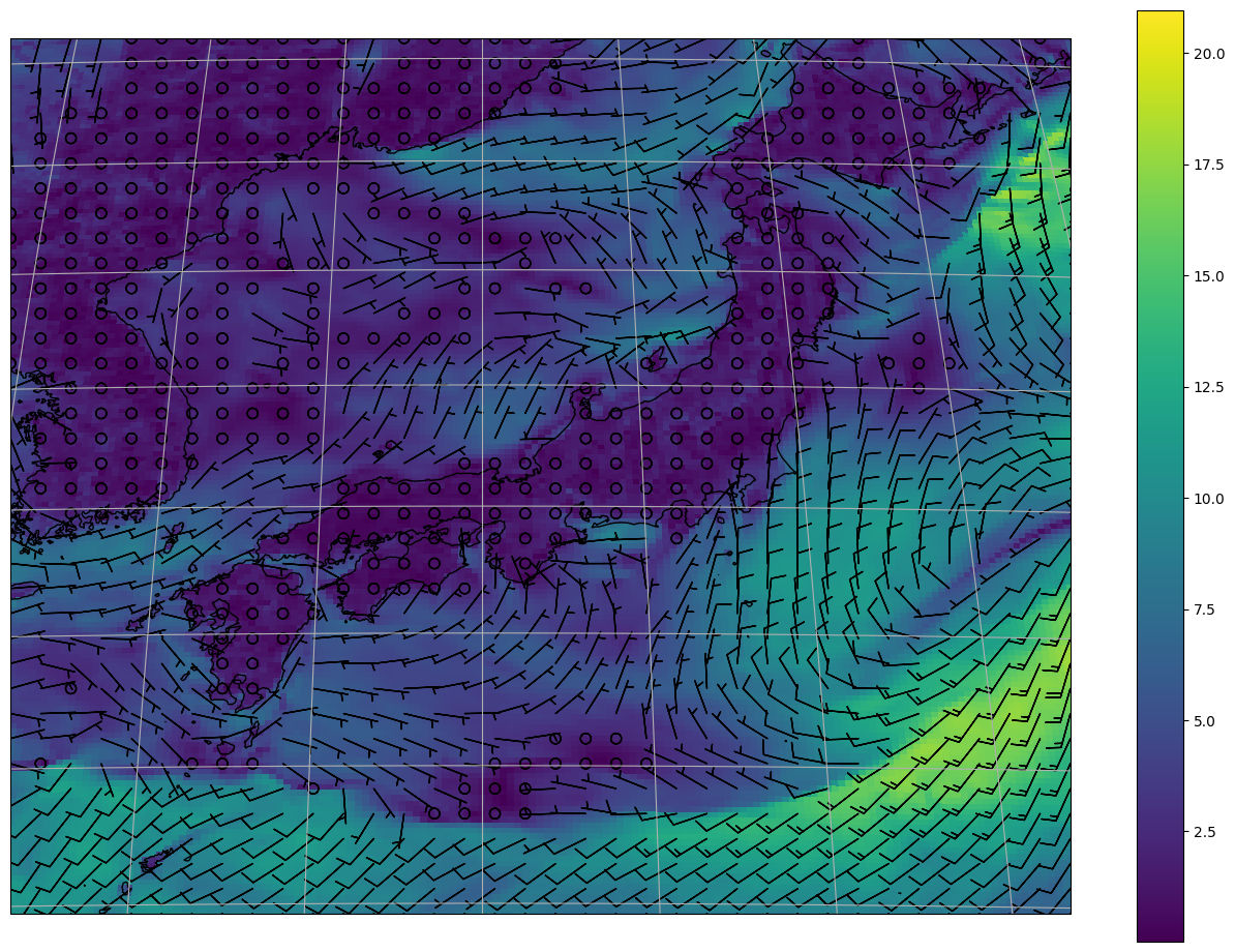
barbs でもまったくおんなじ:
 1 # -*- coding: utf-8 -*-
 2 import os
 3 import sys
 4 import pygrib
 5 import numpy as np
 6 import cartopy.crs as ccrs
 7 import cartopy.feature as cfeature
 8 from cartopy.mpl.ticker import LongitudeFormatter, LatitudeFormatter
 9 import matplotlib.pyplot as plt
10
11
12 def _read(srcfn):
13     src = pygrib.open(srcfn)
14     for s in src:
15         yield s.level, (s.name, s.parameterName), s.validDate, s.latlons(), s.values
16     src.close()
17
18
19 def main(gpv):
20     key_u, key_v = "U component of wind", "V component of wind"
21     data = {}
22     inivd, inilev = None, None
23     for level, yk, vd, latlons, values in _read(gpv):
24         if key_u in yk and key_u not in data:
25             data[key_u] = latlons, values
26             if inivd is None:
27                 inivd, inilev = vd, level
28         if key_v in yk and key_v not in data:
29             data[key_v] = latlons, values
30             if inivd is None:
31                 inivd, inilev = vd, level
32         if len(data) == 2:
33             break
34     (lats, lons), values_u = data[key_u]
35     _, values_v = data[key_v]
36     X, Y = lons[0,:], lats[:,0]
37     #
38     fig = plt.figure()
39     fig.set_size_inches(16.53, 11.69)
40     crs = ccrs.Geostationary(X.mean())
41     ax1 = fig.add_subplot(projection=crs)
42     ext = [X.min() + 7, X.max() - 5, Y.min() + 5, Y.max() - 2]
43     ax1.set_extent(ext, ccrs.PlateCarree())
44     CS = ax1.pcolormesh(
45         X, Y,
46         np.sqrt(values_u**2 + values_v**2),
47         transform=ccrs.PlateCarree(), shading="auto")
48     rs = (int((ext[1] - ext[0]) * 2), int((ext[3] - ext[2]) * 2))
49     ax1.barbs(
50         X, Y,
51         values_u, values_v,
52         transform=ccrs.PlateCarree(),
53         regrid_shape=rs)
54     ax1.coastlines(resolution="10m")
55     ax1.gridlines()
56     plt.colorbar(CS, ax=ax1)
57     #ax1.add_feature(cfeature.OCEAN)
58     #ax1.add_feature(cfeature.LAND)
59
60     plt.savefig("{}_{}_p{}_{}_ba.png".format(
61         os.path.basename(gpv), str(inivd).partition(":")[0], inilev, "wind"),
62         bbox_inches="tight")
63     #plt.show()
64
65
66 if __name__ == '__main__':
67     # 入力は "Z__C_RJTD_20210514000000_MSM_GPV_Rjp_L-pall_FH00-15_grib2.bin" など。
68     main(sys.argv[1])
streamplot は、このタイプの可視化はここ10年以内でやっと天気予報でも目にするようになった例のヤツ:
 1 # -*- coding: utf-8 -*-
 2 import os
 3 import sys
 4 import pygrib
 5 import numpy as np
 6 import cartopy.crs as ccrs
 7 import cartopy.feature as cfeature
 8 from cartopy.mpl.ticker import LongitudeFormatter, LatitudeFormatter
 9 import matplotlib.pyplot as plt
10
11
12 def _read(srcfn):
13     src = pygrib.open(srcfn)
14     for s in src:
15         yield s.level, (s.name, s.parameterName), s.validDate, s.latlons(), s.values
16     src.close()
17
18
19 def main(gpv):
20     key_u, key_v = "U component of wind", "V component of wind"
21     data = {}
22     inivd, inilev = None, None
23     for level, yk, vd, latlons, values in _read(gpv):
24         if key_u in yk and key_u not in data:
25             data[key_u] = latlons, values
26             if inivd is None:
27                 inivd, inilev = vd, level
28         if key_v in yk and key_v not in data:
29             data[key_v] = latlons, values
30             if inivd is None:
31                 inivd, inilev = vd, level
32         if len(data) == 2:
33             break
34     (lats, lons), values_u = data[key_u]
35     _, values_v = data[key_v]
36     X, Y = lons[0,:], lats[:,0]
37     #
38     fig = plt.figure()
39     fig.set_size_inches(16.53, 11.69)
40     crs = ccrs.Geostationary(X.mean())
41     ax1 = fig.add_subplot(projection=crs)
42     ext = [X.min() + 7, X.max() - 5, Y.min() + 5, Y.max() - 2]
43     ax1.set_extent(ext, ccrs.PlateCarree())
44     mag = np.sqrt(values_u**2 + values_v**2)
45     ax1.streamplot(
46         X, Y,
47         values_u, values_v,
48         color=mag,
49         transform=ccrs.PlateCarree())
50     ax1.coastlines(resolution="10m")
51     ax1.gridlines()
52
53     plt.savefig("{}_{}_p{}_{}_sp.png".format(
54         os.path.basename(gpv), str(inivd).partition(":")[0], inilev, "wind"),
55         bbox_inches="tight")
56     #plt.show()
57
58
59 if __name__ == '__main__':
60     # 入力は "Z__C_RJTD_20210514000000_MSM_GPV_Rjp_L-pall_FH00-15_grib2.bin" など。
61     main(sys.argv[1])
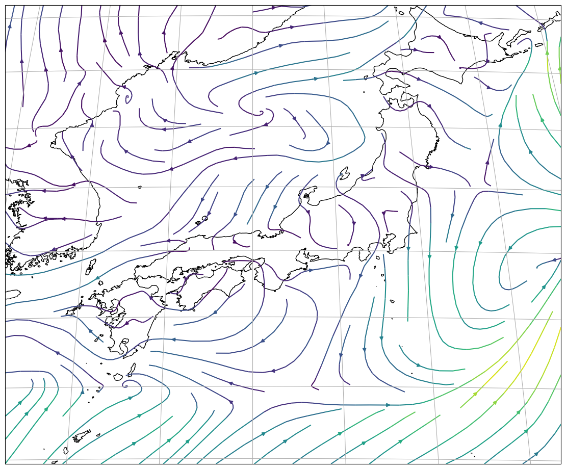
こちらはなぜかスケールの問題は自動的に解決されてるが、まぁこちらは quiver と違って生のベクトルを描画するのではないので、まぁ当然か…。
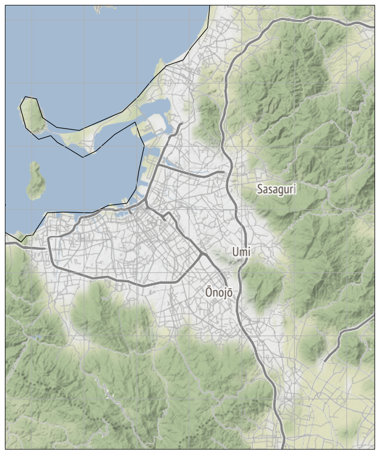
cartopy らしいこと、として目を引くのはやっぱこれかなと思う:
 1 # -*- coding: utf-8 -*-
 2 import os
 3 import sys
 4 import pygrib
 5 import numpy as np
 6 import cartopy.crs as ccrs
 7 import cartopy.feature as cfeature
 8 from cartopy.io.img_tiles import Stamen
 9 import matplotlib.pyplot as plt
10
11
12 def _read(srcfn):
13     src = pygrib.open(srcfn)
14     for s in src:
15         yield (s.name, s.parameterName), s.validDate, s.latlons(), s.values
16     src.close()
17
18
19 def main(gpv):
20     keys = [
21         "Low cloud cover", "Medium cloud cover", "High cloud cover",
22         "Total precipitation"]
23     data = {}
24     inivd = None
25     for yk, vd, latlons, values in _read(gpv):
26         for key in keys:
27             if key in yk and key not in data:
28                 data[key] = latlons, values
29                 if inivd is None:
30                     inivd = vd
31         if len(data) == len(keys):
32             break
33     values = {}
34     for key in keys:
35         (lats, lons), values[key] = data[key]
36     X, Y = lons[0,:], lats[:,0]
37     #
38     tiler = Stamen('terrain-background')
39     mercator = tiler.crs
40     fig = plt.figure()
41     fig.set_size_inches(16.53, 11.69)
42     ax1 = fig.add_subplot(projection=mercator)
43     ext = [X.min() + 7, X.max() - 5, Y.min() + 5, Y.max() - 2]
44     ax1.add_image(tiler, 6, alpha=0.5)
45     ax1.set_extent(ext, ccrs.PlateCarree())
46     for key in keys:
47         if "cloud" in key:
48             cmap = plt.get_cmap("gray")
49         else:
50             cmap = plt.get_cmap("Blues")
51             values[key][np.where(values[key] == 0)] = np.nan
52         ax1.pcolormesh(
53             X, Y,
54             values[key],
55             transform=ccrs.PlateCarree(),
56             shading="auto", alpha=0.3,
57             cmap=cmap)
58     ax1.coastlines(resolution="10m")
59     ax1.gridlines()
60     #ax1.add_feature(cfeature.OCEAN)
61     #ax1.add_feature(cfeature.LAND)
62
63     plt.savefig("{}_{}_{}.png".format(
64         os.path.basename(gpv), str(inivd).partition(":")[0], "cloudcover"),
65         bbox_inches="tight")
66     #plt.show()
67
68
69 if __name__ == '__main__':
70     # 入力は "Z__C_RJTD_20210514000000_MSM_GPV_Rjp_Lsurf_FH00-15_grib2.bin" など。
71     main(sys.argv[1])
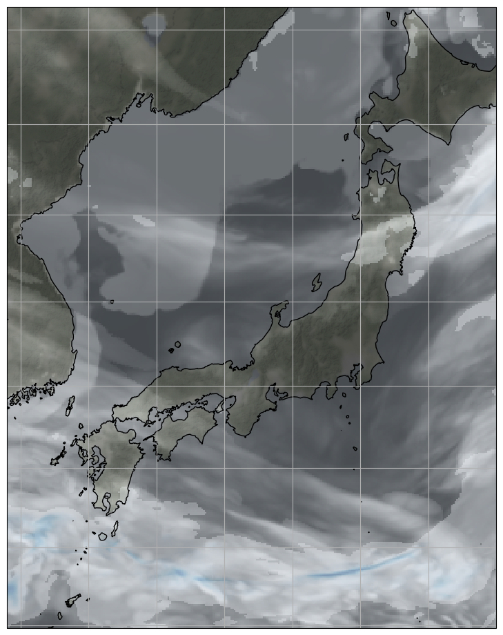
ワタシのサイトの愛読者、なんてのはこの世にはそうそう存在しないはずだが、それでも何かの間違いでワタシのサイトで「Stamen」に心当たりがある人は正解。openlayers の話でこれを扱ってる。openlayers で出来ることを matplotlib で出来るとは何事だ、てことな。
すなわち:
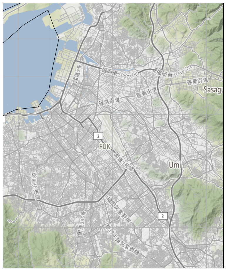
38 tiler = Stamen('toner-background')
とすればこう(ただしalphaは微調整した):
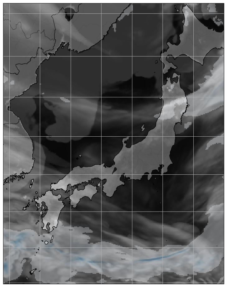
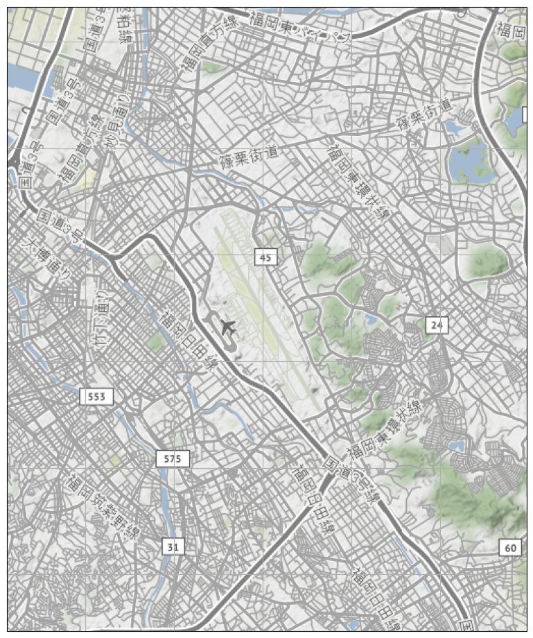
38 tiler = Stamen('toner')
とすればこう(同じくalphaは微調整した):

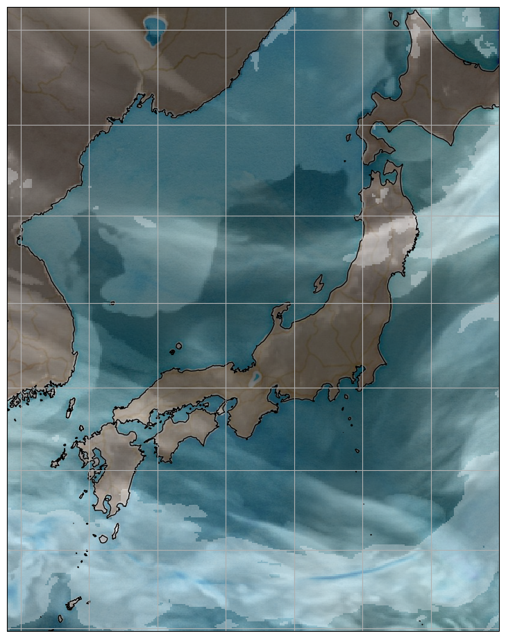
38 tiler = Stamen('watercolor')
とすればこう(同じくalphaは微調整した):
なお、ここまで見せてきたものはいわゆる「地図に対応付け可能なグリッドデータの可視化」であり、「GIS」の一面だけを利用しているわけだ。というか端的に言って「背景に地図を描画する」ことしかしてない。
matplotlib の一番のユーザが要は「行列データを駆使する人たち」なので、ここまでの紹介でほとんど満足できてしまう人たちはかなり多いと思う。けれどもこれを「GIS ソフトウェア」と考えた場合はこれでは不十分で、GIS に少しでも触れたことがある人なら「ジオメトリ描画は出来るの、出来ないの」が気になるのではないだろうか。たとえばこんなね:
 1 # -*- coding: utf-8 -*-
 2 import numpy as np
 3 import pyproj
 4 import matplotlib.pyplot as plt
 5 import cartopy.crs as ccrs
 6 import cartopy.feature as cfeature
 7 from cartopy.io.img_tiles import Stamen
 8 from shapely.geometry import LineString
 9
10
11 def main():
12     _arps = {
13         "RJCJ": (141.666447, 42.794475),
14         "RJFF": (130.450686, 33.585942),
15         "RCBS": (118.359197, 24.427892),
16         "ZPPP": (102.743536, 24.992364),
17     }
18     # 同じ PROJ の「geodesic」に基づく、同じ目的の「Geodesic」が、pyproj では
19     # Geod、cartopy には Geodesic として提供されているが、後者のほうがより薄い
20     # ラッパーに徹していて、pyproj 版のほうが便利。(npts は pyproj の方にしかない。)
21     geod = pyproj.Geod(ellps="WGS84")
22     ps, pd = _arps["RJCJ"], _arps["ZPPP"]
23     intp = list(geod.npts(ps[0], ps[1], pd[0], pd[1], 20))
24     trip_ls = LineString(
25         [(ps[0], ps[1])] + intp + [(pd[0], pd[1])])
26     #
27     tiler = Stamen('terrain')
28     mercator = tiler.crs
29     fig = plt.figure()
30     fig.set_size_inches(16.53, 11.69)
31     ax1 = fig.add_subplot(projection=mercator)
32     ax1.set_extent([100.0, 150.0, 22.4, 47.6], ccrs.PlateCarree())
33     ax1.add_image(tiler, 7, alpha=0.9)
34     ax1.coastlines()  #resolution="10m")
35     ax1.gridlines()
36     #
37     ax1.add_geometries(
38         [trip_ls], ccrs.PlateCarree(), facecolor='none', edgecolor='r')
39     #
40     plt.savefig("exam_add_geometries_01.png", bbox_inches="tight")
41
42
43
44 if __name__ == '__main__':
45     main()
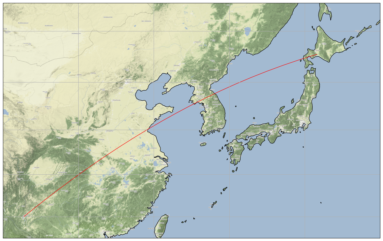
GEOS な幾何学的演算、たとえば交差を求めたりとか、あるいはポリゴンの重なりを計算したりとかして、それで得られた geometry を描画する、みたいなことね。
あと、念の為…。add_image に渡している2つ目の引数は無論ズームレベルに対応するもので、’http://tile.stamen.com/{self.style}/{z}/{x}/{y}.png’ の「z」ね(self.style が「terrain」など)。このズームレベルについて「良きに計らってくれる」メカニズムはないので、自分で選ぶ必要があるし、ワタシにとってはお馴染みの問題「タイル取得に失敗する」も起こる。まぁソースコード修正を試みるとか、「お静かに(穏健に)使う」とかで回避することになろうね、要は領域(bounding box)が大きい場合に複数タイルを一気にお取り寄せるハメになる場合に、トチるのである、しかるにそうならんように使う、てこった。(なお、cache=True の振る舞いは明らかに設計ミス。ダウンロード失敗を永続化しやがんのね、こいつ。修正してえ…。あとで考えよう、リトライの振る舞いも考えたいし。)
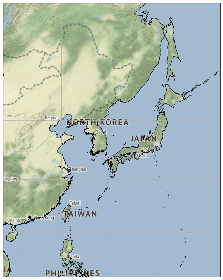
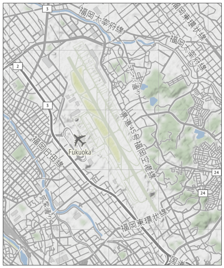
ともあれ:
 1 # -*- coding: utf-8 -*-
 2 import numpy as np
 3 import matplotlib.pyplot as plt
 4 import cartopy.crs as ccrs
 5 from cartopy.io.img_tiles import Stamen
 6
 7
 8 def main():
 9     clon, clat = (130.450686, 33.585942)  # RJFF
10     #
11     zlmax = 18
12     for zl in range(4, zlmax + 1):
13         exp = 360. / 2**zl
14         tiler = Stamen('terrain', cache=True)
15         mercator = tiler.crs
16         fig = plt.figure()
17         fig.set_size_inches(16.53, 11.69)
18         ax1 = fig.add_subplot(projection=mercator)
19         ax1.set_extent(
20             [clon - exp, clon + exp, clat - exp, clat + exp],
21             ccrs.PlateCarree())
22         ax1.add_image(tiler, zl, alpha=0.9)
23         ax1.coastlines(resolution="10m")
24         ax1.gridlines()
25         #
26         plt.savefig(
27             "exam_stamen_terrain_zl{:02d}__.png".format(zl),
28             bbox_inches="tight")
29         plt.close(fig)
30
31
32
33 if __name__ == '__main__':
34     main()
インフラが不完全だとタイル境界の扱いを自分で考えなければならないこともある(つまり境界にぴったり収まらない部分をクリピングするとかそういうこと)が、そうした裏方作業は全部 cartopy.io.image_tiles の責務としてやってくれる。
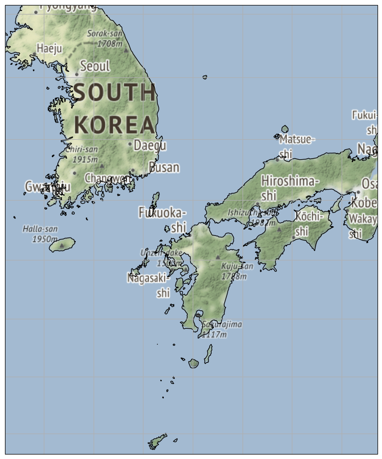
「cache=True」時の振る舞いを理想のものに修正すれば、タイル取得に「失敗したことがあって」も、繰り返せばいずれは全部成功するはず。けどワタシはまだ成功してない、ので、とりあえずz17までの絵:
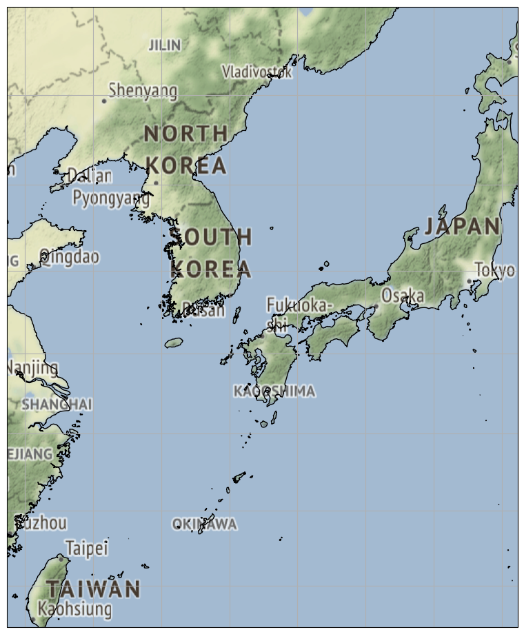
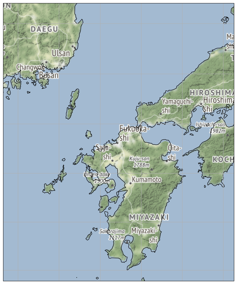
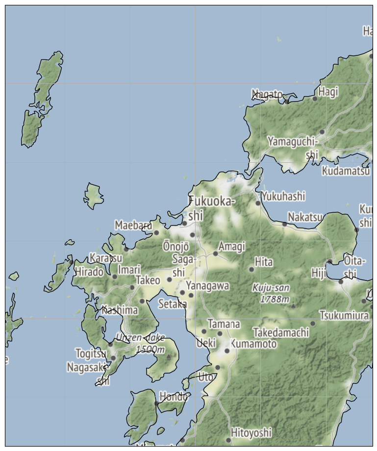
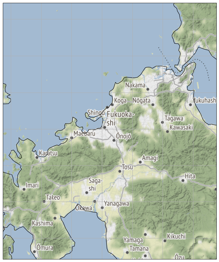
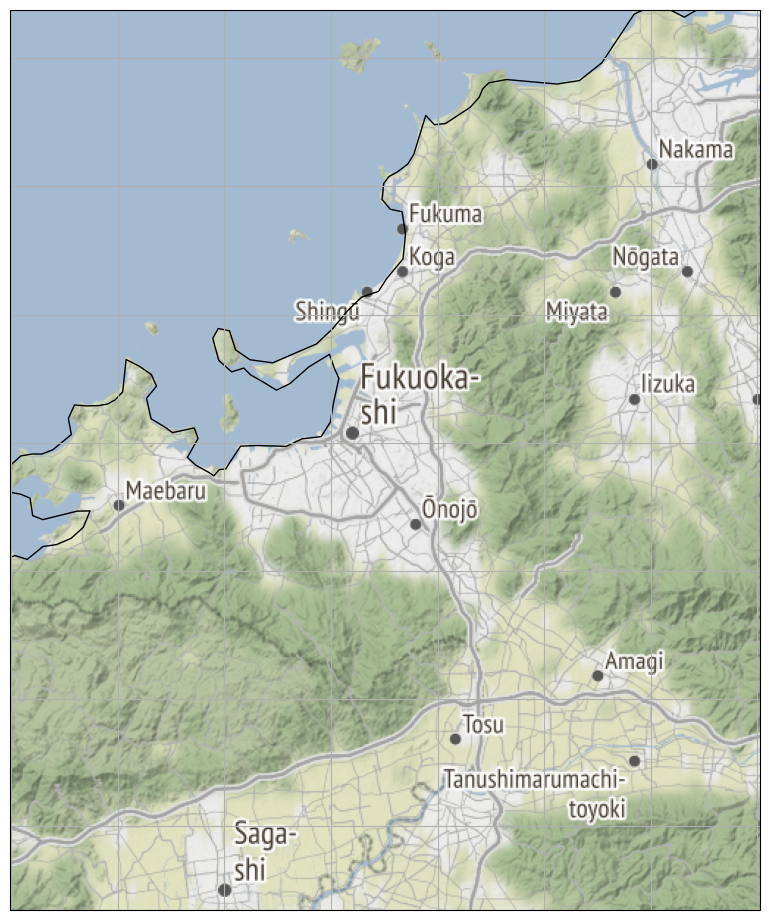
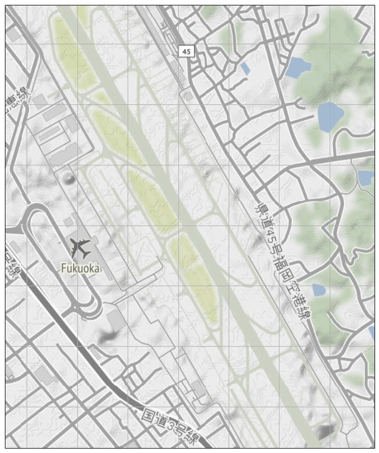

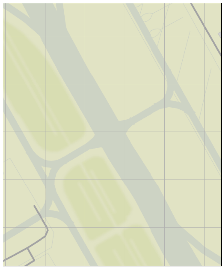
あ…、違うな…。確かにローカル側のキャッシュの問題も考える必要はあって、cartopy のそれは間違いなくダメなんだけれど、「404」なのだもの、これはサーバ側にタイルが出来上がってないんだわ。
mapnik でローカル PC にマップサーバを立てる検証をしたことがあったの思い出したわ。そういやリクエストに応じてタイルが「育っていく」ように構築する決断が出来るわけよね。「予めすべてのタイルを作っておく」んではなく。つまり、使う人が多い地域のタイルは出来上がってる可能性が高く、人気のない地域のタイルは、自分が最初のアクセスとなる確率が高く、その場合にまさに 404 になる。てことだった気がする。これはまぁどうしようもない。(待つしかない。)
2021-05-18 12:00追記:
二点追記。
ひとつ目。アトリビューションを付与してくれる機能がないんだよね、cartopy.io.img_tiles に。どうすりゃいいんだろうかこれ。無論 matplotlib の範疇で set_title とかで描けばいい、ってテクニカルな部分はまぁそれでいいけどね、「アトリビューションとしてこれを必ず書くべし」というのが決まりの地図サービスにおいて、そうであることの知識が cartopy.io.img_tiles に埋め込まれてないのが、ちょっと弱ったことだなぁと。上のワタシの描いた地図には
Map tiles by Stamen Design, under CC BY 3.0. Data by OpenStreetMap, under ODbL.
Map tiles by Stamen Design, under CC BY 3.0. Data by OpenStreetMap, under CC BY SA.
みたいなことを書いておかないといけないのだが、openlayers だとこのアトリビューション付与も機能として提供されてるんだよね。せめて文字列として返す機能だけでも入れといてくんないかなぁ、と思った。
二つ目は、はっきりいってわかる人は言わなくてもわかることなので、蛇足もしくは「野暮」かとも思うんだけれど、一応「目を引く」といって紹介するからには、言っといたほうがいいんだろうなと思ったこと。「Stamen」だけじゃないよ。
openlayers から類推できる人はすぐに「出来るに決まってる」とわかるはずなの、これ。サーバが違うだけで、インターフェイスが統一されてるからこそ、てことだよ:
 1 # -*- coding: utf-8 -*-
 2 import numpy as np
 3 import matplotlib.pyplot as plt
 4 import cartopy.crs as ccrs
 5 from cartopy.io.img_tiles import GoogleTiles
 6
 7
 8 def main():
 9     clon, clat = (130.450686, 33.585942)  # RJFF
10     #
11     zlmax = 18
12     for zl in range(4, zlmax + 1):
13         exp = 360. / 2**zl
14         tiler = GoogleTiles(
15             style='satellite',
16             url=('https://mts0.google.com/vt/lyrs={style}'
17                  '@177000000&hl=ja&src=api&x={x}&y={y}&z={z}&s=G'),
18             cache=True)
19         mercator = tiler.crs
20         fig = plt.figure()
21         fig.set_size_inches(16.53, 11.69)
22         ax1 = fig.add_subplot(projection=mercator)
23         ax1.set_extent(
24             [clon - exp, clon + exp, clat - exp, clat + exp],
25             ccrs.PlateCarree())
26         ax1.add_image(tiler, zl, alpha=0.9)
27         ax1.coastlines(resolution="10m")
28         ax1.gridlines()
29         #
30         plt.savefig(
31             "exam_googletiles_satellite_zl{:02d}.png".format(zl),
32             bbox_inches="tight")
33         plt.close(fig)
34
35
36
37 if __name__ == '__main__':
38     main()
ほかにも MapQuest とかも使える。
2021-05-24追記:
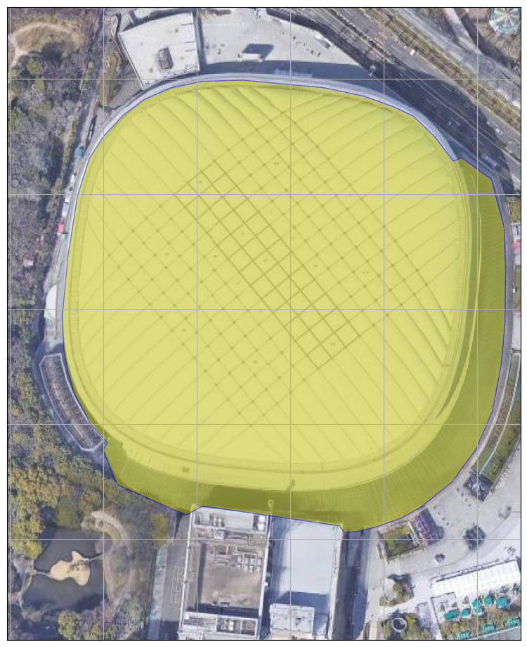
「add_geometries」の実例として挙げたものが、少しだけ一足飛びだったかもしれないと思った。「Great Circle」を求める問題なのだから GIS としては相当の基礎ではあったけれど、「geometry を演算で求めてそれを描画」の「求める」部分が、そもそも「ジオメトリ描画」という基礎にとっては少し邪魔だ、と。ので、もっと直接的な例、すなわち、「既に目的のジオメトリは手持ち」だとする場合の例:
 1 # -*- coding: utf-8 -*-
 2 import shapely.wkt
 3 import numpy as np
 4 import matplotlib.pyplot as plt
 5 import cartopy.crs as ccrs
 6 from cartopy.io.img_tiles import GoogleTiles
 7
 8
 9
10 # This polygon data was extracted from www.openstreetmap.org,
11 # the data is made available under ODbL.
12 _TOKYODOME_POLYGON = shapely.wkt.loads(
13     "POLYGON ((139.7513598 35.7064612, \
14     139.7515235 35.7064901, \
15     139.7517468 35.7064952, \
16     139.7521794 35.7064623, \
17     139.7523926 35.7064262, \
18     139.7525588 35.7063778, \
19     139.7526593 35.7063386, \
20     139.7527745 35.706248, \
21     139.7528709 35.7061439, \
22     139.7529162 35.7061581, \
23     139.7530749 35.7060648, \
24     139.753143 35.7058579, \
25     139.7531508 35.705673, \
26     139.7531475 35.7054376, \
27     139.7531262 35.705252, \
28     139.7530789 35.7050554, \
29     139.7529928 35.7048943, \
30     139.7528655 35.7047525, \
31     139.7526958 35.7046419, \
32     139.7525916 35.7045943, \
33     139.7524667 35.7045587, \
34     139.7523944 35.7045434, \
35     139.7523461 35.7045366, \
36     139.7522891 35.704533, \
37     139.7522608 35.7045617, \
38     139.7521553 35.7045742, \
39     139.7518103 35.7046149, \
40     139.7515323 35.7046478, \
41     139.7514454 35.70461, \
42     139.7513705 35.7046338, \
43     139.7512855 35.7046646, \
44     139.7510745 35.7047411, \
45     139.7509984 35.7048903, \
46     139.7510216 35.7049229, \
47     139.7509335 35.7050014, \
48     139.750846 35.7051343, \
49     139.7508066 35.7052455, \
50     139.7507985 35.7052842, \
51     139.7507889 35.70533, \
52     139.75078 35.7054681, \
53     139.7508092 35.7057256, \
54     139.7508613 35.705993, \
55     139.750925 35.7061552, \
56     139.7509995 35.70625, \
57     139.7511073 35.7063438, \
58     139.751219 35.7064118, \
59     139.7513598 35.7064612))")
60
61
62 def main():
63     clon, clat = (139.75186, 35.705438)
64     #
65     zl = 18
66     exp = 360. / 2**zl
67     tiler = GoogleTiles(style='satellite')
68     fig = plt.figure()
69     fig.set_size_inches(16.53, 11.69)
70     ax1 = fig.add_subplot(projection=tiler.crs)
71     ax1.set_extent(
72         [clon - exp, clon + exp, clat - exp, clat + exp],
73         ccrs.PlateCarree())
74     ax1.add_image(tiler, zl, alpha=0.9)
75     #ax1.coastlines(resolution="10m")
76     ax1.add_geometries(
77         [_TOKYODOME_POLYGON], ccrs.PlateCarree(),
78         facecolor='y', edgecolor='b', alpha=0.5)
79     ax1.gridlines()
80     #
81     plt.savefig(
82         "exam_googletiles_satellite_zl{:02d}_TokyoDome.png".format(zl),
83         bbox_inches="tight")
84     plt.close(fig)
85
86
87
88 if __name__ == '__main__':
89     main()