パッケージの、機能まとめあげについての実力把握、的な話。
cartopy が「わっしゃこいつらに依存しちゃるぜ」と表明しているものたちについて、そのカップリングは適切だろうか、みたいなこと。matplotlib との統合は、第一印象の通りかなり綺麗だと思うのだが、他のはどうなんだろうかと。今日はそれらのうち pyshp の話。
時を戻そう。
一連の cartopy ネタの最初の話は「導入」の話であった。実はこの最初の話には大変大きなターニングポイントがあったのである。何かってぇと、「GIS に関するありとあらゆること」を欲しがるのかそうでないのか、である。そして「GIS に関するありとあらゆること」を欲しがる場合に白羽の矢が立つのが(Windows なら)「オールインワン」で、これを手にしておくと「Shapefile もなんのその」を始めとして、geojson だの geotiff だの、ほんとに「GIS と名の付くいろんなこと」ができるようになる。それでもワタシはそれをあえて選ばずに、出来るだけミニマルであろうとして、あのような導入を紹介した。
戻した時を戻そう。
では、今この「ミニマル」導入した cartopy を手にした状態で、「ESRI Shapefile」は楽に扱えるんだろうか、というかそもそも扱えるんだろうか、と。
まず「そもそも扱えるのだろうか」については杞憂で、pyshp は cartopy にとって必須の依存物である。GeoAxes#coastlines が描画する海岸線が、そもそも shapefile である。pip でのインストール時に依存物として(shapelyとともに)一緒にインストールされる。ゆえに、「pyshp を未インストールの状態で cartopy インストールを試みたユーザ」から見ると、「cartopy を入れるだけで ESRI Shapefile を扱えるようになった」ことになる。「全部入り一」を入れることなく。
cartopy は、ダウンロードした shapefile を pyshp でコッソリ展開する、というだけでなくて、cartopy.io.shapereader として機能提供しているが、まずは先に素の pyshp だけで遊んでみようと思う。すぐに遊べる shapefile は cartopy の中にもあるが、それだと面白くないので、国土地理院のものを使うことにしよう。
pyshp のパッケージ構成はちょっと乱暴なものになってて、「pyshp」というパッケージではなくトップレベルの「shapefile.py」というモジュールがインストールされる。ので、例えばこんな感じ:
 1 # -*- coding: utf-8 -*-
 2 import shapefile
 3 import shapely.geometry as sgeom
 4
 5 # shapefile は .shp、.shx、.dbf の三つ組で一つ、なので、
 6 # shapefile.Reader が受け取る「filename」は、拡張子を除いた
 7 # ベース名でも(いずれかの)拡張子を含めたものでもいい。
 8 filename = "polbnda_jpn"
 9 # Source: Geospatial Information Authority of Japan website
10 #         (https://www.gsi.go.jp/kankyochiri/gm_japan_e.html)
11 reader = shapefile.Reader(filename)
12
13 #
14 for shape_record in reader.iterShapeRecords():
15     print(shape_record.record.as_dict(), sgeom.shape(shape_record.shape))
1 {'f_code': 'FA001', 'coc': 'JPN', 'nam': 'Hokkai Do', 'laa': 'Sapporo Shi', 'pop': 1930496, 'ypc': 2014, 'adm_code': '01100', 'salb': 'UNK', 'soc': 'JPN'} POLYGON ((141.449798583984 43.16333389282232, 141.447692871094 43.15726852416991, 141.453994750977 43.14046859741209, 141.455291748047 43.1246681213379, 141.445098876953 43.10206604003907, 141.457901000977 43.09420013427731, 141.459701538086 43.09960174560549, 141.465194702148 43.10086822509771, 141.467300415039 43.09886550903316, 141.473999023438 43.09700012207031, 141.474105834961 43.09506607055661, 141.475799560547 43.09033203125001, 141.473999023438 43.08653259277337, 141.471694946289 43.08366775512697, 141.473892211914 43.07513427734381, 141.47200012207 43.07026672363278, 141.483901977539 43.06100082397457, 141.489700317383 43.05846405029296, 141.496795654297 43.05879974365229, 141.498001098633 43.05059814453129, 141.500900268555 43.05146789550777, 141.505905151367 43.02173233032233, 141.496795654297 43.02360153198237, 141.486297607422 43.02326583862303, 141.487701416016 43.01826858520511, 141.489501953125 43.0150680541992, 141.484603881836 43.01306533813484, 141.482803344727 43.00773239135741, 141.480697631836 43.00320053100589, 141.477905273438 42.99946594238283, 141.479995727539 42.99613189697268, 141.479690551758 42.9908676147461, 141.46940612793 42.9772682189941, 141.464599609375 42.96466827392582, 141.463104248047 42.95446777343754, 141.457794189453 42.94566726684572, 141.460296630859 42.94406509399408, 141.457702636719 42.94253540039056, 141.435806274414 42.92513275146483, 141.430999755859 42.91986465454098, 141.429397583008 42.91833496093746, 141.421997070313 42.91500091552731, 141.417404174805 42.90886688232424, 141.414001464844 42.89606857299796, 141.421905517578 42.8921318054199, 141.420791625977 42.89086532592769, 141.414199829102 42.88966751098632, 141.407501220703 42.89033508300781, 141.402404785156 42.89093399047854, 141.39680480957 42.88919830322266, 141.395294189453 42.8912658691406, 141.38850402832 42.89133453369144, 141.376998901367 42.891731262207, 141.371795654297 42.89186477661133, 141.371505737305 42.89199829101557, 141.369400024414 42.88800048828129, 141.362594604492 42.88346862792968, 141.358596801758 42.87806701660159, 141.352294921875 42.87553405761717, 141.347900390625 42.87500000000001, 141.335403442383 42.87106704711913, 141.332305908203 42.87146759033204, 141.321105957031 42.87333297729489, 141.317092895508 42.87779998779301, 141.311904907227 42.88639831542974, 141.30549621582 42.88733291625981, 141.300003051758 42.88586807250977, 141.293701171875 42.88426589965823, 141.286804199219 42.87440109252928, 141.282196044922 42.87433242797853, 141.273895263672 42.87133407592771, 141.259201049805 42.86579895019528, 141.254196166992 42.86560058593746, 141.256301879883 42.86073303222661, 141.257202148438 42.8518676757813, 141.253005981445 42.84400177001954, 141.246795654297 42.84080123901372, 141.24479675293 42.84053421020514, 141.241195678711 42.83653259277342, 141.239700317383 42.83086776733402, 141.2373046875 42.82873153686523, 141.235992431641 42.82180023193362, 141.232803344727 42.82159805297853, 141.231994628906 42.8149337768555, 141.226303100586 42.81393432617195, 141.219802856445 42.80879974365234, 141.221801757813 42.8058662414551, 141.224899291992 42.80093383789058, 141.229293823242 42.79846572875982, 141.231201171875 42.79280090332033, 141.22200012207 42.78839874267579, 141.199493408203 42.7850685119629, 141.189605712891 42.78693389892585, 141.179992675781 42.78499984741214, 141.174102783203 42.7859992980957, 141.170593261719 42.78293228149412, 141.162200927734 42.78160095214842, 141.156600952148 42.78620147705078, 141.141494750977 42.78946685791018, 141.136001586914 42.79753112792967, 141.133895874023 42.80400085449224, 141.126892089844 42.8047981262207, 141.121795654297 42.80806732177728, 141.11360168457 42.81280136108398, 141.105392456055 42.81706619262701, 141.093505859375 42.82386779785156, 141.100296020508 42.8281326293945, 141.098693847656 42.83653259277342, 141.094802856445 42.84273529052733, 141.103500366211 42.84799957275391, 141.099304199219 42.85400009155273, 141.099395751953 42.86086654663094, 141.10090637207 42.8680686950684, 141.106506347656 42.87273406982416, 141.10530090332 42.87860107421883, 141.100692749023 42.88426589965823, 141.091995239258 42.88093185424799, 141.084899902344 42.88066864013668, 141.080093383789 42.88593292236326, 141.068298339844 42.8849983215332, 141.049697875977 42.88473129272462, 141.039993286133 42.88613128662108, 141.038101196289 42.89333343505863, 141.035995483398 42.89646530151369, 141.034301757813 42.90560150146484, 141.030792236328 42.9098014831543, 141.027206420898 42.91360092163094, 141.03450012207 42.91986465454098, 141.041793823242 42.93379974365232, 141.047897338867 42.94073104858402, 141.053192138672 42.95299911499023, 141.048706054688 42.95373153686521, 141.044692993164 42.9567337036133, 141.033493041992 42.96073532104494, 141.026901245117 42.96206665039063, 141.022598266602 42.96486663818364, 141.013900756836 42.96620178222661, 141.010101318359 42.97159957885743, 141.0068969726559 42.97926712036128, 141.001495361328 42.97906875610346, 141.001403808594 42.98173141479486, 140.998596191406 42.98693466186522, 140.996795654297 42.99160003662107, 140.993698120117 42.9941329956055, 140.996795654297 43.0004005432129, 140.998306274414 43.00086593627929, 140.999603271484 43.00320053100589, 141.000396728516 43.01313400268551, 140.996795654297 43.01693344116214, 140.99560546875 43.01720046997072, 140.991607666016 43.02313232421879, 140.994598388672 43.02619934082028, 140.996795654297 43.02613449096679, 140.998397827148 43.02606582641603, 141.01139831543 43.03406524658204, 141.016494750977 43.03333282470697, 141.021896362305 43.03426742553712, 141.030395507813 43.04140090942383, 141.0366058349609 43.04426574707031, 141.038696289063 43.04713439941407, 141.044296264648 43.05126571655268, 141.045501708984 43.06146621704096, 141.048599243164 43.06673431396481, 141.058197021484 43.06906509399406, 141.065505981445 43.08406829833979, 141.062103271484 43.08653259277337, 141.060195922852 43.08919906616212, 141.06999206543 43.09280014038094, 141.066390991211 43.0974655151367, 141.063095092773 43.10340118408204, 141.064193725586 43.11153411865229, 141.070693969727 43.10946655273444, 141.075500488281 43.11859893798832, 141.078094482422 43.11826705932617, 141.082397460938 43.11853408813484, 141.085998535156 43.1184005737305, 141.091400146484 43.12099838256842, 141.102401733398 43.11633300781247, 141.104705810547 43.1184005737305, 141.108200073242 43.12013244628911, 141.111404418945 43.11600112915041, 141.121795654297 43.11100006103523, 141.123397827148 43.10993194580083, 141.13330078125 43.10720062255859, 141.133193969727 43.10426712036134, 141.135498046875 43.09453201293946, 141.141693115234 43.09519958496094, 141.152297973633 43.09320068359376, 141.152694702148 43.09019851684567, 141.15690612793 43.08966827392579, 141.161193847656 43.0914001464844, 141.166595458984 43.09433364868164, 141.166900634766 43.09626770019534, 141.17170715332 43.0993995666504, 141.173904418945 43.10393142700201, 141.17790222168 43.10746765136717, 141.18310546875 43.11460113525386, 141.186904907227 43.12046432495117, 141.2014007568359 43.12419891357423, 141.201904296875 43.12613296508793, 141.195495605469 43.13153457641602, 141.191802978516 43.13333511352539, 141.1903991699219 43.13560104370124, 141.188491821289 43.13639831542969, 141.187606811523 43.14086532592773, 141.224594116211 43.16073226928713, 141.226806640625 43.15933227539059, 141.2299041748049 43.15753173828131, 141.238098144531 43.15280151367188, 141.246795654297 43.15886688232419, 141.248199462891 43.15973281860349, 141.283294677734 43.13446807861327, 141.298904418945 43.14139938354488, 141.300201416016 43.14120101928706, 141.309600830078 43.14533233642576, 141.31559753418 43.14759826660161, 141.32470703125 43.14913177490231, 141.328796386719 43.14973449707031, 141.333099365234 43.1493339538574, 141.331695556641 43.1506652832031, 141.334197998047 43.15053558349612, 141.334503173828 43.15266799926764, 141.337493896484 43.1549339294434, 141.341995239258 43.15613174438477, 141.341705322266 43.15813446044922, 141.343292236328 43.15813446044922, 141.34489440918 43.16166687011719, 141.347595214844 43.16033554077149, 141.352798461914 43.16426849365229, 141.351593017578 43.16693115234377, 141.354095458984 43.16986846923829, 141.355392456055 43.17366409301756, 141.360702514648 43.17699813842772, 141.371795654297 43.17380142211908, 141.375503540039 43.17279815673826, 141.387496948242 43.17386627197274, 141.393005371094 43.18000030517581, 141.403305053711 43.1903991699219, 141.405807495117 43.19033432006842, 141.40950012207 43.18659973144527, 141.407501220703 43.18460083007808, 141.399993896484 43.1781311035156, 141.398803710938 43.17393493652341, 141.404098510742 43.17066574096683, 141.418304443359 43.1724662780762, 141.424102783203 43.16986846923829, 141.425094604492 43.16933441162114, 141.426895141602 43.16986846923829, 141.429092407227 43.17093276977541, 141.434295654297 43.16986846923829, 141.434600830078 43.16586685180656, 141.436996459961 43.16226577758792, 141.439300537109 43.16246795654301, 141.448699951172 43.16780090332026, 141.449798583984 43.16333389282232))
2    ...(snip)...
3 {'f_code': 'FA001', 'coc': 'JPN', 'nam': 'Aichi Ken', 'laa': 'UNK', 'pop': -99999999, 'ypc': 0, 'adm_code': 'UNK', 'salb': 'UNK', 'soc': 'JPN'} POLYGON ((136.811904907227 34.99609374999999, 136.805953979492 34.99999999999998, 136.800445556641 35.00362014770514, 136.804092407227 35.00770187377925, 136.808822631836 35.0125694274902, 136.810241699219 35.0134353637695, 136.816604614258 35.01674270629877, 136.819198608398 35.01720046997072, 136.821670532227 35.01763534545896, 136.821685791016 35.01293563842768, 136.821685791016 35.01031875610352, 136.821670532227 35.00800323486335, 136.821166992188 35.00740432739261, 136.817581176758 35.00324630737303, 136.815002441406 34.99999999999998, 136.811904907227 34.99609374999999))
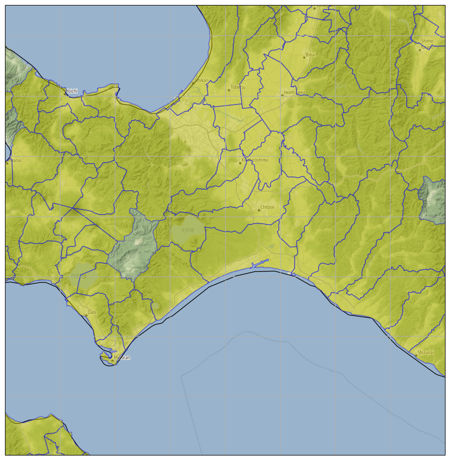
しかるに、このようなことが出来るのであろうと:
 1 # -*- coding: utf-8 -*-
 2 import numpy as np
 3 import pyproj
 4 import matplotlib.pyplot as plt
 5 import cartopy.crs as ccrs
 6 from cartopy.io.img_tiles import Stamen
 7 import shapefile
 8 import shapely.geometry as sgeom
 9
10
11 def main():
12     # shapefile は .shp、.shx、.dbf の三つ組で一つ、なので、
13     # shapefile.Reader が受け取る「filename」は、拡張子を除いた
14     # ベース名でも(いずれかの)拡張子を含めたものでもいい。
15     filename = "polbnda_jpn"
16     # Source: Geospatial Information Authority of Japan website
17     #         (https://www.gsi.go.jp/kankyochiri/gm_japan_e.html)
18     reader = shapefile.Reader(filename)
19
20     #
21     targs = {}
22     for shape_record in reader.iterShapeRecords():
23         attr = shape_record.record.as_dict()
24         if attr["nam"] == "Hokkai Do":
25             targs[attr["laa"]] = sgeom.shape(shape_record.shape)
26     tiler = Stamen('terrain')
27     fig = plt.figure()
28     fig.set_size_inches(16.53, 11.69)
29     ax1 = fig.add_subplot(projection=tiler.crs)
30     ax1.set_extent([140.5, 142.5, 42.0, 43.5], ccrs.PlateCarree())
31     ax1.add_image(tiler, 10)
32     ax1.coastlines(resolution="10m")
33     ax1.gridlines()
34     #
35     ax1.add_geometries(
36         [g for k, g in targs.items()], ccrs.PlateCarree(),
37         facecolor='y', edgecolor='b', alpha=0.5)
38     #
39     #plt.show()
40     plt.savefig("exam_add_geometries_02.png", bbox_inches="tight")
41
42
43
44 if __name__ == '__main__':
45     main()
今日の本題は、「素の shapefile モジュール」をちょっとラップしている「cartopy.io.shapereader」。こちらは、使い方は大差なさげなんだけれど、おそらく「fiona は pyshp より速くてウマイのだぜ、そっちを使うのもおんなじ感じで使えるんだぜぃ」てことなんだと思う。「fiona がインストールされているかどうかに応じて、cartopy.io.shapereader.Reader は BasicReader だったり FionaReader だったりする。つまり、fiona をインストールしていない今のワタシにとっては cartopy.io.shapereader.Reader は pyshp ほぼそのもので、インストールすれば自動的に Fiona になる。これはステキであろう。ゆえに:
 1 # -*- coding: utf-8 -*-
 2 import numpy as np
 3 import pyproj
 4 import matplotlib.pyplot as plt
 5 import cartopy.crs as ccrs
 6 from cartopy.io.img_tiles import Stamen
 7 #import shapefile  # 忘れる。cartopy.io.shapereader があればいいので。
 8 import shapely.geometry as sgeom
 9 from cartopy.io.shapereader import Reader as ShapeReader
10
11
12 def main():
13     # shapefile は .shp、.shx、.dbf の三つ組で一つ、なので、
14     # shapefile.Reader が受け取る「filename」は、拡張子を除いた
15     # ベース名でも(いずれかの)拡張子を含めたものでもいい。
16     # cartopy.io.shapereader の Reader でもこれは同じ。
17     filename = "polbnda_jpn"
18     # Source: Geospatial Information Authority of Japan website
19     #         (https://www.gsi.go.jp/kankyochiri/gm_japan_e.html)
20     reader = ShapeReader(filename)
21
22     #
23     targs = {}
24     #以下の列挙は cartopy.io.shapereader.Reader#records がそっくり
25     #そのまま。
26     #for shape_record in reader.iterShapeRecords():
27     #    attr = shape_record.record.as_dict()
28     #    if attr["nam"] == "Hokkai Do":
29     #        targs[attr["laa"]] = sgeom.shape(shape_record.shape)
30     for r in reader.records():
31         attr = r.attributes
32         if attr["nam"] == "Hokkai Do":
33             targs[attr["laa"]] = r.geometry
34             # r.bounds も便利だろう。
35
36     tiler = Stamen('terrain')
37     fig = plt.figure()
38     fig.set_size_inches(16.53, 11.69)
39     ax1 = fig.add_subplot(projection=tiler.crs)
40     ax1.set_extent([140.5, 142.5, 42.0, 43.5], ccrs.PlateCarree())
41     ax1.add_image(tiler, 10)
42     ax1.coastlines(resolution="10m")
43     ax1.gridlines()
44     #
45     ax1.add_geometries(
46         [g for k, g in targs.items()], ccrs.PlateCarree(),
47         facecolor='y', edgecolor='b', alpha=0.5)
48     #
49     #plt.show()
50     plt.savefig("exam_add_geometries_03.png", bbox_inches="tight")
51
52
53
54 if __name__ == '__main__':
55     main()
結果の絵は完全に同じ。うん、いい感じだ。少し楽になってる上に、「Fiona インストールの恩恵」をこのままで受けられるってんだから。
なお、その「Fiona」だが、おそらく Windows で「簡単に導入」出来ることを期待することは絶望視しておいた方が無難。GDAL 依存なのだが、問題はこの GDAL なのだ、こいつがありとあらゆるものに依存しまくるので、GDAL を入れることを願うことが、即「あーめんどくせぇ全部だ全部」という安直をトリガーしてしまうことが多い。さて、ワタシは果たして QGIS が必要なのだろうか? 否、必要ない。というかこの「全部入り」は、なんなら「Windows で地図サーバを作れるぜ」てくらいに全部入りなので、これをオーバーキルと言わずしてなんというか。(一応 Fiona, GDAL ともに Christoph Gohlke の Unofficial Windows Binaries for Python Extension Packages に含まれてるので、是が非でも欲しい人は検討してみればいい。GDAL についての注意事項はちゃんと熟読するのだぞ。「全部入り一と一緒に使うべからず」をはじめいくつか書いてる。)
というわけで、ワタシにとっての cartopy.io.shapereader は、「Windows 版においては pyshp でええやんけ」「Unix 版で Fiona 入れてても同じスクリプトでええんやぞ」といううまみだけで、まぁいいかなと。生の pyshp を使うよりもスッキリ書けるしね。
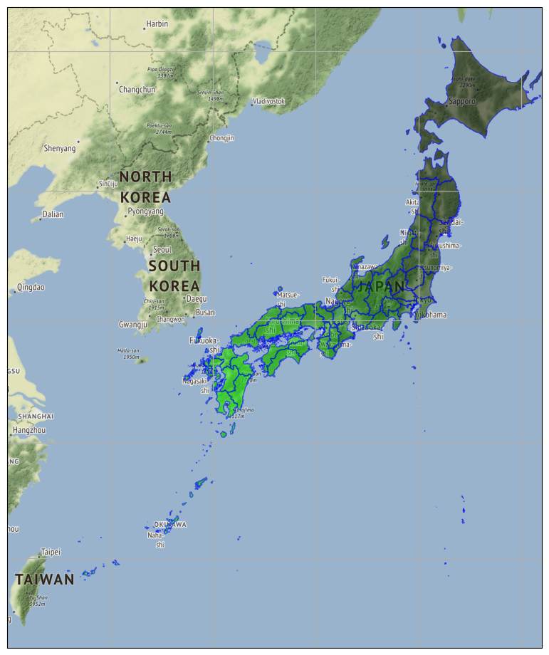
ちなみに国土地理院のものは、どうやら「宮城県全域」みたいなポリゴンは管理されてないみたいなので:
 1 # -*- coding: utf-8 -*-
 2 import numpy as np
 3 import pyproj
 4 import matplotlib.pyplot as plt
 5 import cartopy.crs as ccrs
 6 from cartopy.io.img_tiles import Stamen
 7 import shapely.geometry as sgeom
 8 import shapely.ops as sops
 9 from cartopy.io.shapereader import Reader as ShapeReader
10
11
12 def main():
13     # Source: Geospatial Information Authority of Japan website
14     #         (https://www.gsi.go.jp/kankyochiri/gm_japan_e.html)
15     filename = "polbnda_jpn"
16     reader = ShapeReader(filename)
17
18     #
19     targs = {}
20     for r in reader.records():
21         attr = r.attributes
22         k = attr["nam"]
23         if k not in targs:
24             targs[k] = r.geometry
25         else:
26             targs[k] = sops.cascaded_union([targs[k], r.geometry])
27         # 本題とは関係ないが、"polbnda_jpn" は、案の定というか
28         # ISO-3166-2 の順に収められている。つまり、
29         # if k not in targs が真になるタイミングをカウントしておくと、
30         # それが ISO-3166-2 の都道府県コード(-1)に一致する。
31         # (ただし「初出のものは」。末尾に特殊な地域が47都道府県とは別に
32         # 収められている。)
33
34     tiler = Stamen('terrain')
35     fig = plt.figure()
36     fig.set_size_inches(16.53, 11.69)
37     ax1 = fig.add_subplot(projection=tiler.crs)
38     ax1.set_extent([120.0, 146.0, 21.0, 46.5], ccrs.PlateCarree())
39     ax1.add_image(tiler, 6)
40     #ax1.coastlines(resolution="10m")
41     ax1.gridlines()
42     #
43     ax1.add_geometries(
44         [g for k, g in targs.items()], ccrs.PlateCarree(),
45         facecolor='y', edgecolor='b', alpha=0.5)
46     #
47     #plt.show()
48     plt.savefig("exam_add_geometries_04.png", bbox_inches="tight")
49
50
51
52 if __name__ == '__main__':
53     main()
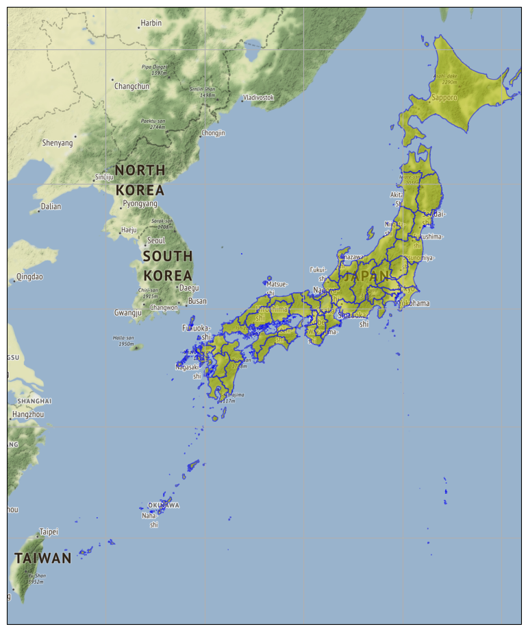
国土地理院以外ので、各都道府県全域ポリゴンを提供してるようなものって、探せばありそうな気がする。探さずこのまま使うのであれば、cascade_union 演算済の状態で予め書き出しておくのがいいだろうね。その場合に shapefile として書き出したい場合、残念だけど cartopy.io.shapewriter なんてものはないので、やるなら pyshp でやることになるだろう。
ただ、どうしても shapefile でなければならないのでない限りは、別に pickle とかでそのまま永続化出来るならそれでいいし、最悪 wkt, wkb の形で永続化するのがお得なこともあるだろうとは思う。そもそも、まぁなんでもそうだけれど「ちゃんとお約束に従わなければ皆の迷惑になる」ことが懸念されるならば、かえってあえて正しいことを目指さない方がいいこともあると思う。人目に触れる可能性がある shapefile を生成したいならこれに従う必要があるんだと思うのよね、これにちゃんと従うのって、世界が破滅するほどに難しいというほどではないにせよ、それなりにヘビィに思える。
実際 pyshp で shapefile を作るのは、コーディングそのものはそう難儀でもないんだけれど、実際やってみて、そしてエラーを喰らってみて思い出したのが、shapefile の制約の強さについてだった。すっかり忘れてたのだけど、一つの shapefile は、異なる geometry_type のものを混在させることが出来ないんだよね。つまり、cascade_union すると POLYGON と MULTIPOLYGON が混在するが、これらは一つの shapefile に収納できない。具体的には、以下はエラーを喰らい、目的を遂行出来ない:
 1 # -*- coding: utf-8 -*-
 2 import shapefile
 3 import shapely.geometry as sgeom
 4 import shapely.ops as sops
 5 from cartopy.io.shapereader import Reader as ShapeReader
 6
 7
 8 def main():
 9     # Source: Geospatial Information Authority of Japan website
10     #         (https://www.gsi.go.jp/kankyochiri/gm_japan_e.html)
11     filename = "polbnda_jpn"
12     reader = ShapeReader(filename)
13     #
14     targs = {}
15     pc = {}
16     for r in reader.records():
17         attr = r.attributes
18         k = attr["nam"]
19         if k not in targs:
20             pc[k] = len(pc) + 1  # ISO-3166-2 の都道府県コードに一致する。
21             targs[k] = r.geometry
22         else:
23             targs[k] = sops.cascaded_union([targs[k], r.geometry])
24
25     # 広く汎用的に皆に使ってもらう「正しい」shapefile を作りたい場合、target 名
26     # も含め
27     #   https://github.com/globalmaps/specifications/raw/master/gmspec-2.2.pdf
28     # に従う必要があるのだと思う。そうしない場合、作られる shapefile は「迷惑なもの」
29     # となるであろう。
30     # shapefile を作ることそのものは、以下に示すように shapefile.Writer で可能
31     # だが、target 名と attributes がどうあるべきなのか私にはわからないので、たぶん
32     # ここで作る shapefile はおそらく「迷惑なもの」だと思う。
33     # (polbnda_jpn が持っている attributes は 'f_code', 'coc', 'nam', 'laa', 'pop',
34     # 'ypc', 'adm_code', 'salb', 'soc' で、これらが何を意味するのかを説明する資料は
35     # ワタシはまだ見つけれてない。わからないなりに「書き出しをお試す」にあたり何を埋めて
36     # おくべきかについて、nam しか思いつかない。とりあえずここではそうしておく。)
37     with shapefile.Writer("polbnda_jpn_prefs") as writer:
38         writer.field("nam", "C", size="25")
39         for k, c in sorted(pc.items(), key=lambda it: (it[1], it[0])):
40             writer.record(k)
41             if targs[k].geom_type == 'MultiPolygon':
42                 parts = [list(p.exterior.coords) for p in list(targs[k])]
43                 writer.polym(parts)
44             else:
45                 parts = list(targs[k].exterior.coords)
46                 writer.poly([parts])
47
48
49 if __name__ == '__main__':
50     main()
こうするしかない:
 1 # -*- coding: utf-8 -*-
 2 import shapefile
 3 import shapely.geometry as sgeom
 4 import shapely.ops as sops
 5 from cartopy.io.shapereader import Reader as ShapeReader
 6
 7
 8 def main():
 9     # Source: Geospatial Information Authority of Japan website
10     #         (https://www.gsi.go.jp/kankyochiri/gm_japan_e.html)
11     filename = "polbnda_jpn"
12     reader = ShapeReader(filename)
13     #
14     targs = {}
15     pc = {}
16     for r in reader.records():
17         attr = r.attributes
18         k = attr["nam"]
19         if k not in targs:
20             pc[k] = len(pc) + 1  # ISO-3166-2 の都道府県コードに一致する。
21             targs[k] = r.geometry
22         else:
23             targs[k] = sops.cascaded_union([targs[k], r.geometry])
24
25     # 広く汎用的に皆に使ってもらう「正しい」shapefile を作りたい場合、target 名
26     # も含め
27     #   https://github.com/globalmaps/specifications/raw/master/gmspec-2.2.pdf
28     # に従う必要があるのだと思う。そうしない場合、作られる shapefile は「迷惑なもの」
29     # となるであろう。
30     # shapefile を作ることそのものは、以下に示すように shapefile.Writer で可能
31     # だが、target 名と attributes がどうあるべきなのか私にはわからないので、たぶん
32     # ここで作る shapefile はおそらく「迷惑なもの」だと思う。
33     # (polbnda_jpn が持っている attributes は 'f_code', 'coc', 'nam', 'laa', 'pop',
34     # 'ypc', 'adm_code', 'salb', 'soc' で、これらが何を意味するのかを説明する資料は
35     # ワタシはまだ見つけれてない。わからないなりに「書き出しをお試す」にあたり何を埋めて
36     # おくべきかについて、nam しか思いつかない。とりあえずここではそうしておく。)
37     with shapefile.Writer("polbnda_jpn_prefs_mp") as writer:
38         writer.field("nam", "C", size="25")
39         for k, c in sorted(pc.items(), key=lambda it: (it[1], it[0])):
40             if targs[k].geom_type == 'MultiPolygon':
41                 writer.record(k)
42                 parts = [list(p.exterior.coords) for p in list(targs[k])]
43                 writer.polym(parts)
44     with shapefile.Writer("polbnda_jpn_prefs_p") as writer:
45         writer.field("nam", "C", size="25")
46         for k, c in sorted(pc.items(), key=lambda it: (it[1], it[0])):
47             if targs[k].geom_type != 'MultiPolygon':
48                 writer.record(k)
49                 parts = list(targs[k].exterior.coords)
50                 writer.poly([parts])
51
52
53 if __name__ == '__main__':
54     main()
何か大きな理由があって shapefile が好きになれなかったんだよね、初めて検証したときに。なんせもうそれって10年前のことなので、もはや理由がなんだったのか忘れていたのだけれど、そうか、そういえばこれが理由だったわ。postgis とかみたいなほかの GIS 関連インフラにない制約だからねこれ。(今回のこれについて言えば、「ISO-3166-2 の都道府県コード順に収められる」という便利な個性まで手放さなければならない、てことだよ。)
そういうわけで、「毎度市区町村単位のポリゴンをお取り寄せて cascade_union する、そのランタイムコストを回避したい」というだけの目的で予め外部化しておく程度の場合は、個人的には shapefile として書き出すのはツーマッチだと考える。それこそ /tmp に書き出しておけばいい、くらいのカジュアルなものなら、pickle とかがいいんではないかしら、って思う。たとえば:
 1 # -*- coding: utf-8 -*-
 2 import io
 3 import pickle
 4 import shapefile
 5 import shapely.geometry as sgeom
 6 import shapely.ops as sops
 7 from cartopy.io.shapereader import Reader as ShapeReader
 8
 9
10 def main():
11     # Source: Geospatial Information Authority of Japan website
12     #         (https://www.gsi.go.jp/kankyochiri/gm_japan_e.html)
13     filename = "polbnda_jpn"
14     reader = ShapeReader(filename)
15     #
16     targs = {}
17     for r in reader.records():
18         attr = r.attributes
19         k = attr["nam"]
20         if k not in targs:
21             pc = len(targs) + 1  # ISO-3166-2 の都道府県コードに一致する。
22             targs[k] = {"g": r.geometry, "pc": pc}
23         else:
24             targs[k]["g"] = sops.cascaded_union([targs[k]["g"], r.geometry])
25     with io.open("polbnda_jpn_prefs.pickle", "wb") as fo:
26         pickle.dump(targs, fo)
27     #with io.open("polbnda_jpn_prefs.pickle", "rb") as fi:
28     #    loaded = pickle.load(fi)
29     #    print(loaded["Tokyo To"]["g"].to_wkt())
30
31 if __name__ == '__main__':
32     main()
無論、誰かしらの通信(交換)相手がいるのなら、msgpack に詰め込むだの色々自由にやればよかろう:
 1 # -*- coding: utf-8 -*-
 2 import io
 3 import json
 4 import msgpack
 5 import shapefile
 6 import shapely.wkb
 7 import shapely.geometry as sgeom
 8 import shapely.ops as sops
 9 from cartopy.io.shapereader import Reader as ShapeReader
10
11
12 def main():
13     # Source: Geospatial Information Authority of Japan website
14     #         (https://www.gsi.go.jp/kankyochiri/gm_japan_e.html)
15     filename = "polbnda_jpn"
16     reader = ShapeReader(filename)
17     #
18     # ジオメトリを wkb として一気にシリアライズすることを前提にしたシンプルな構造で。
19     # つまり
20     # {
21     # "Tokyo To":
22     # b'\x01\x01\x00\x00\x00\x00\x00\x00\x00\x00\x00\xf0?\x00\x00\x00\x00\x00\x00\x00@',
23     # }
24     # のように。せっかく msgpack を使うのだから、てこと。
25     targs = {}
26     pc = {}
27     for r in reader.records():
28         attr = r.attributes
29         k = attr["nam"]
30         if k not in pc:
31             pc[k] = len(targs) + 1  # ISO-3166-2 の都道府県コードに一致する。
32             targs[k] = r.geometry
33         else:
34             targs[k] = sops.cascaded_union(
35                 [targs[k], r.geometry])
36
37     # msgpack でシリアライズするが、geometry は wkb で。
38     # 当たり前だがこの場合、読み手も wkb で書き出されていることを知っている
39     # 必要がある。
40     for k in sorted(pc.keys()):
41         targs[k] = targs[k].to_wkb()
42     with io.open("polbnda_jpn_prefs.bin", "wb") as strm:
43         msgpack.pack(targs, strm)
44     #
45     #unpacked = {
46     #    # to_wkt() の必要性は単に JSONSerializable のため。
47     #    # 内部的に使う際はむしろ to_wkt() は邪魔なので注意。
48     #    k: shapely.wkb.loads(v).to_wkt()
49     #    for k, v in msgpack.unpack(
50     #            io.open("polbnda_jpn_prefs.bin", "rb")).items()}
51     #print(json.dumps(unpacked, indent=4))
52
53
54 if __name__ == '__main__':
55     main()
geojson がいいなら shapely 機能の mapping, shape を駆使して:
 1 # -*- coding: utf-8 -*-
 2 import io
 3 import json
 4 import shapefile
 5 import shapely.geometry as sgeom
 6 import shapely.ops as sops
 7 from cartopy.io.shapereader import Reader as ShapeReader
 8
 9
10 def main():
11     # Source: Geospatial Information Authority of Japan website
12     #         (https://www.gsi.go.jp/kankyochiri/gm_japan_e.html)
13     filename = "polbnda_jpn"
14     reader = ShapeReader(filename)
15     #
16     # GeoJSON の spec(https://geojson.org/geojson-spec.html) に従ってみる。
17     # なお、GeoJSON は obsoleted, replaced by RFC7946 ということになってるが、
18     # RFC として公式に格上げした、という以上の差異はなさそう。ざっと見では
19     # 同じものに見える。https://datatracker.ietf.org/doc/html/rfc7946 参照。
20     targs = dict(type="FeatureCollection", features=[])
21     lastk = None
22     for r in reader.records():
23         attr = r.attributes
24         k = attr["nam"]
25         if k != lastk:
26             targs["features"].append(
27                 dict(
28                     type="feature",
29                     geometry=sgeom.mapping(r.geometry),
30                     properties={"nam": k}))
31         else:
32             targs["features"][-1]["geometry"] = sgeom.mapping(sops.cascaded_union(
33                 [sgeom.shape(targs["features"][-1]["geometry"]), r.geometry]))
34         lastk = k
35     print(json.dumps(targs, indent=4))
36
37
38 if __name__ == '__main__':
39     main()
みたいに出来るけれども、ほんとに相手がいてその相手が geojson 以外を許さない場合以外は、ここまでする必要はなかろう。そもそもさっきまでやってた shapefile としてや pickle として書き出したのと結果が違う。末尾に東京都と愛知県の特殊領域が分離された状態になる。そういうわけで、どうしても geojson にしなければならないケースであっても、内部形式まで geojson フォーマットに従おうとするのではなくて、扱いやすい形式(先にやってたように、nam をキーとする辞書など)で保持しておいて、必要になってから geojson に変換するアプローチを採るべきだろう。(→ちょっと考え直したので後ろのほうの「2021-06-10追記」参照。)
都道府県ごとに色を変えたい、なんてことはすぐにしそうになりそうなので、今のうち遊んでおこう:
 1 # -*- coding: utf-8 -*-
 2 import numpy as np
 3 import pyproj
 4 import matplotlib.pyplot as plt
 5 import cartopy.crs as ccrs
 6 from cartopy.io.img_tiles import Stamen
 7 import shapely.geometry as sgeom
 8 import shapely.ops as sops
 9 from cartopy.io.shapereader import Reader as ShapeReader
10
11
12 def main():
13     # Source: Geospatial Information Authority of Japan website
14     #         (https://www.gsi.go.jp/kankyochiri/gm_japan_e.html)
15     filename = "polbnda_jpn"
16     reader = ShapeReader(filename)
17     #
18     targs = {}
19     pc = {}
20     for r in reader.records():
21         attr = r.attributes
22         k = attr["nam"]
23         if k not in targs:
24             pc[k] = len(pc) + 1  # ISO-3166-2 の都道府県コードに一致する。
25             targs[k] = r.geometry
26         else:
27             targs[k] = sops.cascaded_union([targs[k], r.geometry])
28
29     tiler = Stamen('terrain')
30     fig = plt.figure()
31     fig.set_size_inches(16.53, 11.69)
32     ax1 = fig.add_subplot(projection=tiler.crs)
33     ax1.set_extent([120.0, 146.0, 21.0, 46.5], ccrs.PlateCarree())
34     ax1.add_image(tiler, 6)
35     ax1.gridlines()
36     #
37     for k, g in targs.items():
38         ax1.add_geometries(
39             [g], ccrs.PlateCarree(),
40             facecolor='#00{:02x}00'.format(int(255 * (pc[k] / 47))),
41             edgecolor='b', alpha=0.5)
42     #plt.show()
43     plt.savefig("exam_add_geometries_05.png", bbox_inches="tight")
44
45
46 if __name__ == '__main__':
47     main()
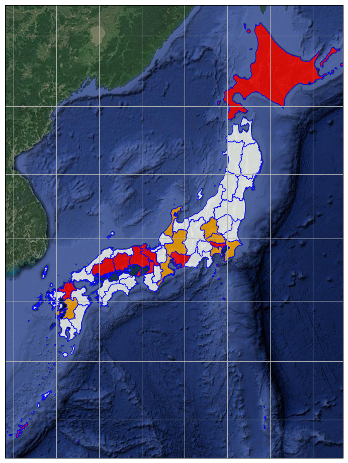
いいね。こういうことが出来るなら、例えば COVID-19 感染状況のステージで色分けする、なんてことも出来る、てこった:
ついでなので、こうした可視化では良くやる、「都道府県の代表点を中心とした円の大きさで何かを表現する」ヤツもやってみておく:
  1 # -*- coding: utf-8 -*-
  2 import numpy as np
  3 import pyproj
  4 import matplotlib.pyplot as plt
  5 import cartopy.crs as ccrs
  6 from cartopy.io.img_tiles import Stamen
  7
  8
  9 _PREFCODE = {
 10     '北海道': 1,
 11     '青森県': 2,
 12     '岩手県': 3,
 13     '宮城県': 4,
 14     '秋田県': 5,
 15     '山形県': 6,
 16     '福島県': 7,
 17     '茨城県': 8,
 18     '栃木県': 9,
 19     '群馬県': 10,
 20     '埼玉県': 11,
 21     '千葉県': 12,
 22     '東京都': 13,
 23     '神奈川県': 14,
 24     '新潟県': 15,
 25     '富山県': 16,
 26     '石川県': 17,
 27     '福井県': 18,
 28     '山梨県': 19,
 29     '長野県': 20,
 30     '岐阜県': 21,
 31     '静岡県': 22,
 32     '愛知県': 23,
 33     '三重県': 24,
 34     '滋賀県': 25,
 35     '京都府': 26,
 36     '大阪府': 27,
 37     '兵庫県': 28,
 38     '奈良県': 29,
 39     '和歌山県': 30,
 40     '鳥取県': 31,
 41     '島根県': 32,
 42     '岡山県': 33,
 43     '広島県': 34,
 44     '山口県': 35,
 45     '徳島県': 36,
 46     '香川県': 37,
 47     '愛媛県': 38,
 48     '高知県': 39,
 49     '福岡県': 40,
 50     '佐賀県': 41,
 51     '長崎県': 42,
 52     '熊本県': 43,
 53     '大分県': 44,
 54     '宮崎県': 45,
 55     '鹿児島県': 46,
 56     '沖縄県': 47,
 57 }
 58
 59
 60 def main():
 61     # Source: Geospatial Information Authority of Japan website
 62     #         (https://www.gsi.go.jp/kankyochiri/gm_japan_e.html)
 63     filename = "polbnda_jpn"
 64     reader = ShapeReader(filename)
 65
 66     #
 67     targs = {}
 68     pc = {}
 69     for r in reader.records():
 70         attr = r.attributes
 71         k = attr["nam"]
 72         if k not in targs:
 73             pc[k] = len(pc) + 1
 74             targs[k] = r.geometry
 75         else:
 76             targs[k] = sops.cascaded_union([targs[k], r.geometry])
 77
 78     tiler = Stamen('terrain')
 79     fig = plt.figure()
 80     fig.set_size_inches(16.53, 11.69)
 81     ax1 = fig.add_subplot(projection=tiler.crs)
 82     ax1.set_extent([126.0, 146.5, 25.0, 46.5], ccrs.PlateCarree())
 83     ax1.add_image(tiler, 6)
 84     ax1.gridlines()
 85     #
 86     def _centroid(geom):
 87         # 東京と沖縄が特に顕著なのだが、たとえば「東京の~の値は…」というビジュアラ
 88         # イズを、円の大きさで表現したいとして、その際に円の中心として「東京都」という
 89         # union したポリゴン の centroid を使うならば、当然これは海上になる。そう
 90         # ではなくて、実用上は陸にある代表点を使えれば十分なわけだ。都道府県庁の緯度
 91         # 経度を管理できているならそれを使えばいいけれど、polbnda_jpn だけで求める
 92         # つもりならば、どうにか島嶼部を除いたポリゴンに基づく centroid を求めたい、
 93         # てこと。つまり MULTIPOLYGON 内の POLYGON で面積が最も大きいものの
 94         # centroid を求めればよかろう、てこと。
 95         if geom.geom_type == 'Polygon':
 96             return geom.centroid
 97         maxarea = 0
 98         selected = None
 99         for p in list(geom):
100             if p.area > maxarea:
101                 selected = p
102                 maxarea = p.area
103         return selected.centroid
104     #
105     #
106     from shapely.geometry import asPolygon
107     from cartopy.geodesic import Geodesic
108     wgs84 = Geodesic()
109     import io, csv
110     tpositive_sum = {}
111     r = csv.reader(io.open("prefectures.csv", encoding="utf-8"))
112     next(r)
113     for line in r:
114         # 最新の値のみ。(testedPositive は累積値なので今回の場合は目的のもの。)
115         tpositive_sum[_PREFCODE[line[3]]] = int(line[5])
116     #
117     for k, g in targs.items():
118         # tpositive_sum の大きさに応じた円。
119         ct = _centroid(g)
120         ci = asPolygon(wgs84.circle(ct.x, ct.y, 0.75 * tpositive_sum[pc[k]]))
121         ax1.add_geometries(
122             [ci], ccrs.PlateCarree(),
123             facecolor='r',
124             edgecolor='b', alpha=0.5)
125     #
126     #plt.show()
127     plt.savefig("exam_add_geometries_06.png", bbox_inches="tight")
128
129
130
131 if __name__ == '__main__':
132     import os
133     import urllib.request
134     import shutil
135     if not os.path.exists("prefectures.csv"):
136         cont, msg = urllib.request.urlretrieve(
137             "https://toyokeizai.net/sp/visual/tko/covid19/csv/prefectures.csv")
138         shutil.move(cont, "prefectures.csv")
139     main()
(3)で「pyproj の Geod の方が便利」と言ったけれど、cartopy.geodesic.Geodesic には、これまた便利な「circle」があるのよねぇ、こいつぁ弱ったな。(地図に円を描くのって、実はとても高等な演算。)ともあれ、こんな絵が描ける:
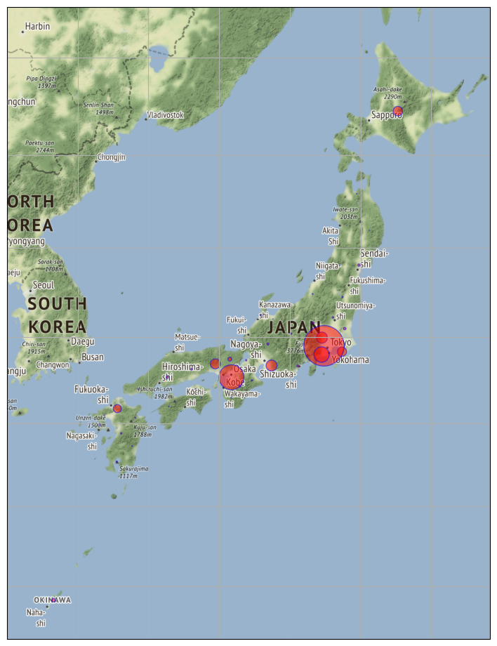
スケーリングをかなり意識的にやらないとわかりやすいビジュアライズとはなりえない。サボったのでもちろんその通り「何これわかりにくい」可視化と化してる。けど「頑張れば出来る」の道を拓く、という目的では、ひとまずこれで満足しなはれ。
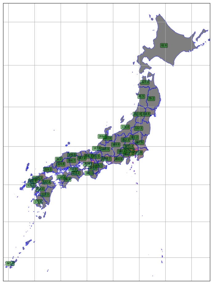
pyproj と cartopy.geodesic.Geodesic の関係についてはもう一つ、geometry_area_perimeter がある。m^2 での面積を求めてくれる機能で、これがあれば例えば人口密度の可視化が出来ることになる。話のついでに GeoAxes#text なんぞも駆使してみるとして:
  1 # -*- coding: utf-8 -*-
  2 import csv
  3 import numpy as np
  4 import pyproj
  5 import matplotlib.pyplot as plt
  6 import matplotlib.font_manager
  7 from matplotlib.transforms import offset_copy
  8 import cartopy.crs as ccrs
  9 from cartopy.io.img_tiles import Stamen
 10 import shapely.geometry as sgeom
 11 import shapely.ops as sops
 12 from cartopy.io.shapereader import Reader as ShapeReader
 13
 14
 15 # wikipedia より。
 16 _POPUL_TSV = """\
 17 1\t東京都\t13000-1\t13,515,271\t13,960,236\t+3.29\t2021年1月1日
 18 2\t神奈川県\t14000-7\t9,126,214\t9,216,009\t+0.98\t2020年9月1日
 19 3\t大阪府\t27000-8\t8,839,469\t8,815,082\t-0.28\t2020年11月1日
 20 4\t愛知県\t23000-6\t7,483,128\t7,538,701\t+0.74\t2020年11月1日
 21 5\t埼玉県\t11000-1\t7,266,534\t7,342,682\t+1.05\t2020年12月1日
 22 6\t千葉県\t12000-6\t6,222,666\t6,281,869\t+0.95\t2021年1月1日
 23 7\t兵庫県\t28000-3\t5,534,800\t5,434,645\t-1.81\t2021年1月1日
 24 8\t北海道\t01000-6\t5,381,733\t5,231,685\t-2.79\t2020年11月30日
 25 9\t福岡県\t40000-9\t5,101,556\t5,108,038\t+0.13\t2020年9月1日
 26 10\t静岡県\t22000-1\t3,700,305\t3,613,788\t-2.34\t2021年1月1日
 27 11\t茨城県\t08000-4\t2,916,976\t2,852,499\t-2.21\t2021年1月1日
 28 12\t広島県\t34000-6\t2,843,990\t2,793,470\t-1.78\t2020年11月1日
 29 13\t京都府\t26000-2\t2,610,353\t2,566,341\t-1.69\t2021年1月1日
 30 14\t宮城県\t04000-2\t2,333,899\t2,290,915\t-1.84\t2021年1月1日
 31 15\t新潟県\t15000-2\t2,304,264\t2,195,068\t-4.74\t2021年1月1日
 32 16\t長野県\t20000-0\t2,098,804\t2,031,795\t-3.19\t2021年1月1日
 33 17\t岐阜県\t21000-5\t2,031,903\t1,975,397\t-2.78\t2020年9月1日
 34 18\t栃木県\t09000-0\t1,974,255\t1,930,000\t-2.24\t2021年1月1日
 35 19\t群馬県\t10000-5\t1,973,115\t1,924,116\t-2.48\t2021年1月1日
 36 20\t岡山県\t33000-1\t1,921,525\t1,880,772\t-2.12\t2021年1月1日
 37 21\t福島県\t07000-9\t1,914,039\t1,820,949\t-4.86\t2021年1月1日
 38 22\t三重県\t24000-1\t1,815,865\t1,768,632\t-2.60\t2020年9月1日
 39 23\t熊本県\t43000-5\t1,786,170\t1,734,231\t-2.91\t2021年1月1日
 40 24\t鹿児島県\t46000-1\t1,648,177\t1,587,785\t-3.66\t2021年1月1日
 41 25\t沖縄県\t47000-7\t1,433,566\t1,460,427\t+1.87\t2021年1月1日
 42 26\t滋賀県\t25000-7\t1,412,916\t1,412,095\t-0.06\t2021年1月1日
 43 27\t山口県\t35000-1\t1,404,729\t1,339,003\t-4.68\t2021年1月1日
 44 28\t愛媛県\t38000-8\t1,385,262\t1,323,851\t-4.43\t2021年1月1日
 45 29\t長崎県\t42000-0\t1,377,187\t1,308,277\t-5.00\t2021年1月1日
 46 30\t奈良県\t29000-9\t1,364,316\t1,321,250\t-3.16\t2021年1月1日
 47 31\t青森県\t02000-1\t1,308,265\t1,228,730\t-6.08\t2020年12月1日
 48 32\t岩手県\t03000-7\t1,279,594\t1,209,457\t-5.48\t2021年1月1日
 49 33\t大分県\t44000-1\t1,166,338\t1,124,309\t-3.60\t2020年11月1日
 50 34\t石川県\t17000-3\t1,154,008\t1,129,362\t-2.14\t2020年12月1日
 51 35\t山形県\t06000-3\t1,123,891\t1,062,239\t-5.49\t2021年1月1日
 52 36\t宮崎県\t45000-6\t1,104,069\t1,062,180\t-3.79\t2021年1月1日
 53 37\t富山県\t16000-8\t1,066,328\t1,033,981\t-3.03\t2020年11月1日
 54 38\t秋田県\t05000-8\t1,023,119\t948,964\t-7.25\t2021年1月1日
 55 39\t香川県\t37000-2\t976,263\t949,357\t-2.76\t2020年9月1日
 56 40\t和歌山県\t30000-4\t963,579\t912,364\t-5.32\t2021年1月1日
 57 41\t山梨県\t19000-4\t834,930\t805,339\t-3.54\t2021年1月1日
 58 42\t佐賀県\t41000-4\t832,832\t808,074\t-2.97\t2021年1月1日
 59 43\t福井県\t18000-9\t786,740\t762,272\t-3.11\t2020年11月1日
 60 44\t徳島県\t36000-7\t755,733\t721,721\t-4.50\t2020年9月1日
 61 45\t高知県\t39000-3\t728,276\t688,583\t-5.45\t2021年1月1日
 62 46\t島根県\t32000-5\t694,352\t665,702\t-4.13\t2021年1月1日
 63 47\t鳥取県\t31000-0\t573,441\t550,651\t-3.97\t2021年1月1日"""
 64
 65
 66 def main():
 67     #
 68     fontprop = matplotlib.font_manager.FontProperties(size=6)
 69     #
 70     popl = {}
 71     reader = csv.reader(_POPUL_TSV.split("\n"), delimiter="\t")
 72     for row in reader:
 73         popl[int(row[2][:2])] = int(row[4].replace(",", ""))
 74
 75     # Source: Geospatial Information Authority of Japan website
 76     #         (https://www.gsi.go.jp/kankyochiri/gm_japan_e.html)
 77     filename = "polbnda_jpn"
 78     reader = ShapeReader(filename)
 79     #
 80     targs = {}
 81     pc = {}
 82     for r in reader.records():
 83         attr = r.attributes
 84         k = attr["nam"]
 85         if k not in targs:
 86             pc[k] = len(pc) + 1  # ISO-3166-2 の都道府県コードに一致する。
 87             targs[k] = r.geometry
 88         else:
 89             targs[k] = sops.cascaded_union([targs[k], r.geometry])
 90
 91     tiler = Stamen('terrain')
 92     fig = plt.figure()
 93     fig.set_size_inches(16.53, 11.69)
 94     ax1 = fig.add_subplot(projection=tiler.crs)
 95     ax1.set_extent([127.0, 146.75, 25.0, 46.25], ccrs.PlateCarree())
 96     #ax1.add_image(tiler, 6)  #タイルと一緒だと読みにくいか?
 97     ax1.gridlines()
 98     #
 99     popud = {}
100     wgs84 = pyproj.Geod(ellps="WGS84")
101     for k, g in targs.items():
102         thearea = abs(wgs84.geometry_area_perimeter(g)[0])  # m^2
103         thearea /= (1000**2)  # km^2
104         popud[k] = popl[pc[k]] / thearea  # 人口密度 [人/km2]
105         #print(popud[k])
106     popudmax = max([v for k, v in popud.items()])
107     #
108     def _centroid(geom):
109         if geom.geom_type == 'Polygon':
110             return geom.centroid
111         maxarea = 0
112         selected = None
113         for p in list(geom):
114             if p.area > maxarea:
115                 selected = p
116                 maxarea = p.area
117         return selected.centroid
118     #
119     # 人口密度の値をテキストとして描画したい、として、これがちょっと特殊。
120     # cartopy のソース配布物内の examples/scalar_data/eyja_volcano.py 参照。
121     # ----------------------------------------------------------------------
122     # Use the cartopy interface to create a matplotlib transform object
123     # for the Geodetic coordinate system. We will use this along with
124     # matplotlib's offset_copy function to define a coordinate system which
125     # translates the text by 2 pixels to the right.
126     # なお、パラメータを省略した ccrs.Geodetic() は WGS84 としての構築。
127     geodetic_transform = ccrs.Geodetic()._as_mpl_transform(ax1)
128     text_transform = offset_copy(geodetic_transform, units='dots', x=2)
129     # ----------------------------------------------------------------------
130     #
131     for k, g in targs.items():
132         c = '#{:02x}0000'.format(int(255 * (popud[k] / popudmax)))
133         ax1.add_geometries(
134             [g], ccrs.PlateCarree(),
135             facecolor=c,
136             edgecolor='b', alpha=0.5)
137         ct = _centroid(g)
138         ax1.text(ct.x, ct.y, "{:.1f}".format(popud[k]),
139                  verticalalignment='center', horizontalalignment='right',
140                  transform=text_transform,
141                  fontproperties=fontprop,
142                  bbox=dict(facecolor='green', alpha=0.5, boxstyle='round')
143         )
144     #plt.show()
145     plt.savefig("exam_add_geometries_07.png", bbox_inches="tight")
146
147
148 if __name__ == '__main__':
149     main()
これの結果はこんな:
「シームレスな機能統合」という意味において「_as_mpl_transform」はなんとも残念なところだが、こういうのはいずれ綺麗に整理されていくことだろう。「pyproj で出来ることが cartopy.geodesic.Geodesic でも出来うるべき」かどうかは、Jeffrey Whitaker と Cartopy プロジェクトの双方の考え方によるだろう。歩み寄るのかそのまま別プロジェクトとして維持されるのか。歩み寄るということは、pyproj が役目を終えることを意味する。どうなるかは見守るしかないんだけど、オープンな議論は残ってたりしないのかしらね? 真剣に探せばきっと見つかるんだろうね…。
2021-05-31追記:
ここでやってる「日本全域を丸ごと収める領域に、日本にある場所を示す文字を描画する」というケースでは問題にはならないのだけれど、描画したいテキストが set_extent で指定した範囲外になりうる場合は注意が必要だとわかった。ほんとに素直に領域外に描画しちゃう。
自力で範囲内にいるかチェックする方法については(6)の中でやった。
まぁ理解は出来なくはないのだけどね、実際箱の外に少しくらいははみ出てもいい、という方が普通は使い勝手がいいから。けど、も少し綺麗にやる手はないもんだろうか?
2021-06-10追記:
「どうしても geojson にしなければならないケースであっても、内部形式まで geojson フォーマットに従おうとするのではなくて、扱いやすい形式で保持しておいて、必要になってから geojson に変換するアプローチを採るべきだろう」と書いたのだけれど、ほかにも色々見ていく中で、ひょっとしたら geojson 流儀に乗っかっておくのは悪くないことかもしれない、と思い始めてる。
「お約束」のどれに従うのがお得か、というのは、規約が乱立していれば当然悩ましい問題で、今の場合、少なくとも「GML 流儀」「OSM 流儀」「OGC 流儀」とともに geojson 流儀がある、ということになるわけなのだが、この geojson 流儀、というのが、python においては「__geo_interface__」として整理されていて、実は「ワタシ」は気付かずにこれの恩恵を受けていたのであった。「「どうしても geojson にしなければならないケースであっても云々」を書いたところに書いたスクリプトが依存した「shapely.geometry.mapping」と「shapely.geometry.shape」が実はこの __geo_interface__ に依拠していて、ゆえに、こういう構築が可能:
 1 import shapely.geometry as sgeom
 2 # __geo_interface__ そのものではなくてその中身だけ与えてもそれに反応する。
 3 g = sgeom.shape({"type": "Point", "coordinates": (143.2, 39.4)})
 4
 5 # __geo_interface__ の本来の姿はこんな:
 6 class MyNanika(object):
 7     # たとえば shapely をなんらかの事情でインストールしたくないとかで
 8     # 自力定義したいとして。
 9     __geo_interface__ = {
10         "type": "Point",
11         "coordinates": (143.2, 39.4),
12         "properties": {"name": "dokoka"}
13         # ほか、オプショナルに bbox, geometry を持てる。
14         # geometry はこれは「type="Feature"」用だろう。
15         # "geometry": inner.__geo_interface__ みたいに
16         # 入れ子構造になることが念頭に置かれた属性。
17     }
18 # shapely.geometry.mapping はこの __geo_interface__ から
19 # 引っ張ってきてくれる。
20 print(sgeom.mapping(MyNanika()))
21 # geojson パッケージをインストールした場合も、dumper はこれを拾う。
22 import geojson
23 print(geojson.dumps(MyNanika()))
PEP-465のように公式 Python に認められたプロトコルではないけれど、shapefile・OSM・geojson のいずれがソースであってもその情報を過不足なく保持出来て、便利に思えるのよね。すなわち「ホームポジション」として結構適切なんじゃないかしらと。