「とっても広域」時のデータを小さくする方法、しばらくやらなくていいかなと思ったんだけど、やりたくなっちゃった。
(7)で、東京に扇状地があることをはじめて知って、是非全体像を、と思って。結構なサイズになる。
まずいい加減にやりたければ「スキップ」でいいんだけれど、やっぱり「ちゃんと」縮小したい。scipy の ndimage.zoom 使うと楽。けどその前に、「ちゃんとしないとどう残念で、ちゃんとするとどうステキか」の効果の確認:
 1 # ...(省略)...
 2 #
 3 import matplotlib
 4 import matplotlib.cm as cm
 5 import matplotlib.pyplot as plt
 6 from matplotlib.colors import LightSource
 7 import scipy.ndimage as ndimage
 8
 9 ls = LightSource(azdeg=180, altdeg=15)
10
11 fig, (ax1, ax2, ax3) = plt.subplots(3)
12
13 rgb = ls.shade(elevs, cm.rainbow)
14 ax1.imshow(rgb)
15 ax1.set_xticks([])
16 ax1.set_yticks([])
17 ax1.set_title("original")
18
19 ax2.imshow(rgb[::3, ::3])
20 ax2.set_xticks([])
21 ax2.set_yticks([])
22 ax2.set_title("simply skip [::3, ::3]")
23
24 rgb = ls.shade(
25     ndimage.zoom(
26         elevs,
27         1. / 3,
28         prefilter=False),
29     cm.rainbow)
30 ax3.imshow(rgb)
31 ax3.set_xticks([])
32 ax3.set_yticks([])
33 ax3.set_title("ndimage.zoom(1 / 3)")
34
35 plt.savefig("t.png", bbox_inches="tight")
36 #
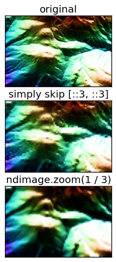
単なるスキップではちょっと「残念」でしょ。ちゃんと zoom で縮小すれば滑らか。いいね?
さて。「大量メモリを使うのを避けたい」がために zoom したいとするならば、converted_loader.py が一個のセルを load してすぐさま zoom して小さくしてしまうのが良いことになるので、converted_loader.py を、「一個ロード後に変換関数を呼び出す」ように改造する:
  1 # -*- coding: utf-8 -*-
  2 try:
  3     # for CPython 2.7
  4     import cPickle as pickle
  5 except ImportError:
  6     # Python 3.x or not CPython
  7     import pickle
  8 import numpy as np
  9
 10
 11 def _calc_pos0(lon_or_lat, lseg):
 12     a = (lon_or_lat % 100) / lseg
 13     b = (a - int(a)) / (1 / 8.)
 14     c = (b / (1 / 10.)) % 10
 15     return (
 16         int(a),
 17         int(b),
 18         int(c),
 19         round((int(a) + int(b) / 8. + int(c) / 8. / 10.) * lseg, 9),
 20         round((int(a) + int(b) / 8. + (int(c) + 1) / 8. / 10.) * lseg, 9))
 21
 22
 23 def _calc_from_latlon(lat, lon):
 24     _fromlat = _calc_pos0(lat, 2/3.)
 25     _fromlon = _calc_pos0(lon, 1.)
 26     return (
 27         "__converted/{}{}/{}{}/{}{}".format(
 28             _fromlat[0], _fromlon[0],
 29             _fromlat[1], _fromlon[1],
 30             _fromlat[2], _fromlon[2]),
 31         (_fromlat[3], _fromlon[3] + 100),
 32         (_fromlat[4], _fromlon[4] + 100))
 33
 34
 35 def load(lat, lon, convert_fun=None):
 36     base, lc, uc = _calc_from_latlon(lat, lon)
 37     shape = (150, 225)
 38     elevs = np.full((shape[1] * shape[0], ), np.nan)
 39
 40     try:
 41         _d = pickle.load(open(base + ".data", "rb"))
 42         _st = _d["startPoint"]
 43         _raw = _d["elevations"]
 44         elevs[_st:len(_raw) + _st] = _raw
 45     except IOError as e:
 46         print(str(e))
 47
 48     elevs = elevs.reshape((shape[0], shape[1]))
 49     elevs = np.flipud(elevs)
 50
 51     if convert_fun:
 52         elevs = convert_fun(elevs)
 53
 54     return elevs, lc, uc
 55
 56
 57 def _load_range0(lc_lat, lc_lon, uc_lat, uc_lon, convert_fun=None):
 58     #
 59     def _stfun(fun, left, right):
 60         if left is None:
 61             return right
 62         return fun((left, right))
 63     #
 64     ydis = (2. / 3 / 8 / 10)
 65     xdis = (1. / 8 / 10)
 66
 67     # adjust startpoint to center of mesh
 68     # (for special boundary case.)
 69     lc_lat = int(lc_lat / ydis) * ydis + ydis / 2.
 70     lc_lon = int(lc_lon / xdis) * xdis + xdis / 2.
 71
 72     ycells = int(np.ceil(uc_lat / ydis) - np.floor(lc_lat / ydis))
 73     xcells = int(np.ceil(uc_lon / xdis) - np.floor(lc_lon / xdis))
 74     result, lc, uc = None, None, None
 75     #
 76     for i in range(ycells):
 77         tmp = None
 78         for j in range(xcells):
 79             e, lc_tmp, uc_tmp = load(
 80                 lc_lat + ydis * i,
 81                 lc_lon + xdis * j,
 82                 convert_fun)
 83             #
 84             if not lc:
 85                 lc = lc_tmp
 86             uc = uc_tmp
 87             #
 88             tmp = _stfun(np.hstack, tmp, e)
 89         #
 90         result = _stfun(np.vstack, result, tmp)
 91     #
 92     return result, lc, uc
 93
 94
 95 def load_range(lc_lat, lc_lon, uc_lat, uc_lon, convert_fun=None):
 96     elevs, lc, uc = _load_range0(
 97         lc_lat, lc_lon, uc_lat, uc_lon,
 98         convert_fun)
 99     X = np.linspace(lc[1], uc[1], elevs.shape[1])
100     Y = np.linspace(lc[0], uc[0], elevs.shape[0])
101     xmin, xmax = np.where(X <= lc_lon)[0][-1], np.where(X >= uc_lon)[0][0]
102     ymin, ymax = np.where(Y <= lc_lat)[0][-1], np.where(Y >= uc_lat)[0][0]
103     return X[xmin:xmax], Y[ymin:ymax], elevs[ymin:ymax, xmin:xmax]
この方法の難点は、最小セルのサイズ(150, 225)が綺麗に割り切れる縮小率でないと困ったことになる点。つまり行列サイズの端数の扱いに困る。最後に一回かけるだけの変換なら問題ない端数でも、あとで結合することになるブロック一つ一つで端数が出ると困る。
これはもう仕方がないと諦めるしかなくて、ここでやるなら、1/3、1/5、1/15、1/25 のいずれかを選ぶしかない。ただ、これは考え方次第。一つのセルごとに 1/3、1/5、1/15、1/25 にしたあとの結合後にさらに zoom すれば良いということもないではないので。(メモリ節約の効果は薄くなるけれど。)
つぅわけで、「武蔵野扇状地」。範囲は「35.565881, 139.256914」~「35.930066, 139.791998」という、かなりの広範囲で、データ削減しない場合、(6555, 9633) という shape になってしまい、処理がいつになっても終わらないことになってしまう。これは (7)の 2×2 = 4 倍くらい。ので、zoom(1/3)でやってみる:
  1 # -*- coding: utf-8 -*-
  2 import numpy as np
  3 import converted_loader
  4 import scipy.ndimage as ndimage
  5
  6 def _zoom(d):
  7     return ndimage.zoom(
  8         d,
  9         1. / 3,
 10         mode="nearest",
 11         prefilter=False)
 12
 13 X, Y, elevs = converted_loader.load_range(
 14     35.565881, 139.256914,
 15     35.930066, 139.791998,
 16     convert_fun=_zoom)
 17
 18 elevs[np.isnan(elevs)] = np.nanmin(elevs)
 19 print(elevs.shape)
 20
 21 #
 22 import matplotlib
 23 import matplotlib.cm as cm
 24 import matplotlib.pyplot as plt
 25 from mpl_toolkits.axes_grid1 import make_axes_locatable
 26
 27 elevs = np.flipud(elevs)
 28
 29 fig, ax = plt.subplots()
 30 fig.set_size_inches(16.53 * 2, 11.69 * 2)
 31
 32 from matplotlib.colors import LightSource
 33 ls = LightSource(azdeg=180, altdeg=15)
 34 rgb = ls.shade(elevs, cm.rainbow)
 35 cs = ax.imshow(elevs)
 36 ax.imshow(rgb)
 37
 38 # create an axes on the right side of ax. The width of cax will be 2%
 39 # of ax and the padding between cax and ax will be fixed at 0.05 inch.
 40 divider = make_axes_locatable(ax)
 41 cax = divider.append_axes("right", size="2%", pad=0.05)
 42 fig.colorbar(cs, cax=cax)
 43
 44 ax.set_xticks([])
 45 ax.set_yticks([])
 46
 47 import matplotlib.font_manager
 48 import matplotlib.patheffects as PathEffects
 49 fontprop = matplotlib.font_manager.FontProperties(
 50     fname="c:/Windows/Fonts/msyh.ttf")
 51 # ----------------
 52
 53 def _latlon2xy(lat, lon):
 54     return (
 55         int((lon - X[0]) / (X[1] - X[0])),
 56         len(Y) - int((lat - Y[0]) / (Y[1] - Y[0])))
 57
 58 font = {
 59     "fontproperties": fontprop,
 60     'color'  : 'white',
 61     'weight' : 'normal',
 62     'size'   : 32,
 63     }
 64 anns = [
 65     ((35.619231, 139.728713), u'大崎駅', (1, 1)),
 66     ((35.714074, 139.771575), u'上野公園', (1, 1)),
 67     ((35.777697, 139.721074), u'赤羽駅', (1, 1)),
 68     ((35.573352, 139.684585), u'光明寺', (1, 1)),
 69     ((35.579399, 139.705936), u'池上本門寺', (1, 1)),
 70     ((35.787986, 139.275881), u'青梅市役所', (1, 1)),
 71     ((35.777588, 139.405050), u'狭山湖', (1, 1)),
 72     #((35.652972, 139.252782), u'八王子城址', (1, 1)),
 73     ((35.593224, 139.730269), u'大森貝塚', (1, 1)),
 74     ((35.603693, 139.646342), u'等々力渓谷', (1, 1)),
 75     ((35.589359, 139.667162), u'多摩川台公園', (1, 1)),
 76     ((35.657406, 139.748189), u'増上寺', (1, 1)),
 77     ((35.611360, 139.561343), u'生田緑地', (1, 1)),
 78     ((35.768790, 139.420645), u'西武プリンスドーム', (1, 1)),
 79     ((35.855762, 139.327961), u'飯野市役所', (1, 1)),
 80     ]
 81
 82 for (lat, lon), ann, (off_y, off_x) in anns:
 83     tx, ty = _latlon2xy(lat, lon)
 84     p = ax.annotate(
 85         ann,
 86         (tx, ty),
 87         (tx + off_x, ty + off_y),
 88         arrowprops=dict(
 89             arrowstyle="->",
 90             connectionstyle="angle",
 91             lw=1
 92             ),
 93         size=10,
 94         ha="center",
 95         path_effects=[
 96             PathEffects.withStroke(linewidth=2, foreground="w")
 97             ],
 98         fontproperties=fontprop)
 99     p.arrow_patch.set_path_effects([
100             PathEffects.Stroke(linewidth=2, foreground="w"),
101             PathEffects.Normal()])
102 #
103 plt.savefig("musashino-senjyochi.pdf", bbox_inches="tight")
104 #
(8.5)で試みた文字入れもやっている。結果はこんな:
Click here to download
おぅ。ざっつ扇状地。とっても扇状地。というか、なんたる大規模な扇状地。富山の黒部の扇状地と違って「肉眼でわかる」ことはなさそうだから、住んでる人も自覚してないだろうなぁ。あぁ、この独特な「狭山丘陵」って、西武ドームがあるとこか…。中学校時代に叔父に連れられて行ったきりだなぁ、当時は当然ドームじゃなくて「西武球場」で。南海ホークスと西武ライオンズの試合、でした。
もっと地名とか情報入れたいんだけどね、東京の海に近くないとこも埼玉も、ワタシ的にかなり未知だもんで。地名入れてもなおピンと来なかったりするんす。
2015-10-10 追記
最初の投稿時点で2箇所の問題があった。
converted_loader.py の、「adjust startpoint to center of mesh」部分が10日に追加した箇所。この調整がない場合、緯度経度がちょうどメッシュ境界だった場合の振る舞いがおかしくなる。
もう一つが、同じく converted_loader.py の最後の行、np.where部分。最初の投稿時点では等号が入っていなかった。これが入っていないと IndexError が起こりうる。